Blog Archives
A Rickety Stairway to SQL Server Data Mining, Part 14.6: Custom Mining Functions
by Steve Bolton
…………In the last installment of this amateur series of mistutorials on SQL Server Data Mining (SSDM), I explained how to implement the Predict method, which controls how the various out-of-the-box prediction functions included with SSDM are populated in custom algorithms. This limits users to returning the same standard columns returned by calls to prediction functions against the nine algorithms that ship with SSDM. The PredictHistogram function, for example, will return a single prediction column, plus columns labeled $Support, $Probability, $AdjustedProbability, $Variance and $StDev, just as it does with the out-of-the-box algorithms. Although we can control the output of the standard prediction functions to return any values we want, it may be more suitable in some cases to specify our own output format with more flexibility. This is where the ability to define your own custom mining functions comes in handy. Another important use case is when you need to perform custom calculations that wouldn’t normally be implemented in standard prediction functions like PredictStDev or PredictSupport. Plug-in programmers could conceivably perform any complicated calculation they like in the Predict method and return it in the results for PredictVariance, but this would be awkward and illogical if the result is not a measure of variance. Thankfully, the SSDM plug-in architecture we’ve been discussing in the past articles includes a mechanism for defining your own custom mining functions, which addresses all of these needs.
…………Aside from the calculation of cumulative statistics, developing a custom mining function is actually quite simple. The development process begins by declaring a public function in your AlgorithmBase class ordained with a MiningAlgorithmClassAttribute, which looks like the attribute declaration in my sample code: <MiningFunction(“My Custom Mining Function Description”)>. The text within the quotation marks will appear in the DESCRIPTION column of the DMSCHEMA_MINING_FUNCTIONS schema rowset, for the row corresponding to the new function. The parameter list can contain variables of your choosing, like the RecordCount integer I use in my sample code for limiting the rows returned by MyCustomMiningFunction, but special rules apply in a few cases. Parameters decorated with the MiningTableColumnRefAttribute or MiningScalarColumnRefAttribute tags must be AttributeGroup objects, such as the <MiningScalarColumnRefAttribute()> TempAttributeGroup AsAttributeGroup declaration in my sample code. I believe MiningTableColumnRefAttribute tags are used for feeding nested tables to custom mining functions, but the PluginModel mining model we’ve been working with in this segment on custom mining algorithms doesn’t have one, nor do I see any benefit in adding one because of the risk of cluttering the tutorial needlessly. MiningScalarColumnRefAttribute, however, is a more common tag that allows you to pass a reference to a specific model column; in the prediction I’ll execute to test the function, I’ll pass a value of “InputStat” to identify the first column in the PluginModel. The Flag attribute can also be used to identify optional flags passed as parameters to the function, as I do in the parameter declaration <Flag()> INCLUDE_COUNT AsBoolean. Apparently, these flags must be Booleans, because I received the following warning in the FUNCTION_SIGNATURE column of DMSCHEMA_MINING_FUNCTIONS whenever I use other data types with a flag I called ATTRIBUTE_NUMBER that I later removed: “Invalid Flag type (must be Boolean) in method MyCustomMiningFunction:ATTRIBUTE_NUMBER.” The algorithm will still deploy correctly if these parameters are set wrong but will return error messages when prediction queries are executed against the custom functions. The parameter list may also include a MiningCase object, which is not exposed to end users and causes SSDM to automatically iterate over the case set supplied in a prediction join, OpenQuery, or other such statement. As we shall see, one of the primary challenges with custom mining functions is to calculate cumulative statistics by iterating over this MiningCase object.
…………You can basically return values you want from your function, but if they’re scalar, they must be declared as System.Object. To return more than one value your only choice is to declare the return type as System.Data.DataTable. If your revised AlgorithmBase code compiles and deploys correctly, then the next time the service starts you should see your choice reflected in the RETURNS_TABLE column of DMSCHEMA_MINING_FUNCTIONS. Note how the query in Figure 1 reflects the name of the method we added to AlgorithmBase in the FUNCTION_Name column, the string from the MiningAlgorithmClassAttribute in the DESCRIPTION and the lists of parameters in FUNCTION_SIGNATURE. Some other standard functions enabled for our sample plug-in are also listed in the results (minus the prediction functions I enabled for the last tutorial, which were removed to shorten the list).
Figure 1: The Custom Mining Function Depicted in DMSCHEMA_MINING_FUNCTIONS

…………Note that the MyCustomMiningFunction is listed twice; this is because it is declared in AlgorithmBase and in SupportedFunction.CustomFunction Base, as part of the array returned by AlgorithmMetadataBase. Removing the function from AlgorithmBase without removing it from SupportedFunction.CustomFunction Base from the array returned by AlgorithmMetadataBase.GetSupportedStandardFunctions led to this error on msmdsrv, when the algorithm failed to initialize: “The data mining algorithm provider (ProgID: 06da68d6-4ef0-4cea-b4dd-1a7c62801ed2) for the Internal_Name_For_My_Algorithm algorithm cannot be loaded. COM error: COM error: DMPluginWrapper; Parameter name: in_FunctionOrdinal Actual value was 10000.” Another “gotcha” you may encounter is the warning that “PREDICTION JOIN is not supported” for a particular mining model when you try to use the function in a query. After many comparisons to the original sample code provided in the plug-in software development kit (SDK) by Bogdan Crivat, one of the original developers of SSDM, I was able to narrow this down to the cases in which the GetCaseIdModeled method of AlgorithmMetadataBase returns True. Simply changing the return value for that method ought to fix the problem. Another common mistake you may encounter while testing custom mining functions is leaving off the ON clause in the PREDICTION JOIN, which may result in this warnng: “Parser: The end of the input was reached.” As renowned SQL Server Analysis Services (SSAS) guru Chris Webb says in his helpful post Error messages in MDX SELECT statements and what they mean, this can also be due to missing parentheses, brackets and semi-colon marks. All of these myriad issues were fairly inconsequential in comparison to those that arose when I debugged the AlgorithmNavigationBase class in A Rickety Stairway to SQL Server Data Mining, Part 14.4: Node Navigation, which is far easier than troubleshooting AlgorithmBase and less difficult by several orders of magnitude than dealing with exceptions in AlgorithmMetadataBase. The biggest challenge I encountered while writing the sample code depicted in Figure 2 was calculating cumulative values across iterations over the MiningCase object, which were problematic to persist.
Figure 2: Sample Code for MyCustomMiningFunction
<MiningFunction(“My Custom Mining Function Description”)>
Public Function MyCustomMiningFunction(InputCase As MiningCase, RecordCount As Integer, <MiningScalarColumnRefAttribute()> TempAttributeGroup As AttributeGroup, <Flag()> INCLUDE_COUNT As Boolean) As System.Data.DataTable
Static CaseCount As UInteger = 0 ‘the 0th case will be the Prepare statement
‘for whatever reason, the first InputCase is always Nothing
‘we can use that opportunity to set up the data table one time only
If IsNothing(InputCase) = True Then
MyCustomMiningFunctionDataTable = New System.Data.DataTable ‘on the first iteration, reset the datatable
MyCustomMiningFunctionDataTable.Columns.Add(“Skewness”, GetType(Double))
MyCustomMiningFunctionDataTable.Columns.Add(“Kurtosis”, GetType(Double))
MyCustomMiningFunctionDataTable.Columns.Add(“ExcessKurtosis“, GetType(Double))
MyCustomMiningFunctionDataTable.Columns.Add(“JBStatistic“, GetType(Double))
If INCLUDE_COUNT = True Then
MyCustomMiningFunctionDataTable.Columns.Add(“TotalRows“, GetType(UInteger))
End If
‘once the data type is set, we can return it one time, in the event of a Prepare statement
‘I will have to double-check later and make sure this statement doesn’t need to execute for each row during Prepared statements
‘Bogdan: “•If the execution is intended for a Prepare statement, it returns an empty string. A Prepare execution must return data that has the same type and schema (in case of tables) with the real result.”
‘so if it is only for a prepare statement, we’d send it back the empty data table?
‘chm: on Context.ExecuteForPrepare: “Determines whether the current query is preparing the execution or it is fully executing. Should only be used in the implementation of custom functions”
If Context.ExecuteForPrepare = True Then
Return MyCustomMiningFunctionDataTable
End If
Else
‘dealing with actual cases; add them to the cumulatives so we
can perform calculations at the end
‘for now we will deal with a single attribute for the sake of simplicity; it would be fairly easy though to extend this to deal with more than one attribute at a time
Try
If CaseCount < RecordCount – 1 Then ‘RecordCount is 1-based, CaseCount is not
‘both variables are 0-based
If CaseCount = 0 Then
ReDim TempSkewnessKurtosisClassArray(0) ‘initialize the arrays one time; this won’t work during the Preparation phase when InputCase = 0, because other variables will be set to 1
ReDim TempDataPointArray(0, RecordCount – 1)
TempSkewnessKurtosisClassArray(0) = New SkewnessKurtosisClass
End If
TempDataPointArray(0, CaseCount) = New DataPointClass
TempDataPointArray(0, CaseCount).DataPoint = InputCase.DoubleValue
TempSkewnessKurtosisClassArray(0).TotalValue = TempSkewnessKurtosisClassArray(0).TotalValue + InputCase.DoubleValue
CaseCount = CaseCount + 1
Else
‘add the last set
If IsNothing(TempSkewnessKurtosisClassArray(0)) Then TempSkewnessKurtosisClassArray(0) = New SkewnessKurtosisClass
TempDataPointArray(0, CaseCount) = New DataPointClass
TempDataPointArray(0, CaseCount).DataPoint = InputCase.DoubleValue
TempSkewnessKurtosisClassArray(0).TotalValue = TempSkewnessKurtosisClassArray(0).TotalValue + InputCase.DoubleValue
CaseCount = CaseCount + 1
‘if we’re on the final case, calculate all of the stats
Dim TempRow As System.Data.DataRow
TempRow = MyCustomMiningFunctionDataTable.NewRow()
TempSkewnessKurtosisClassArray(0).Mean
= SkewnessKurtosisClassArray(0).CalculateAverage(RecordCount, TempSkewnessKurtosisClassArray(0).TotalValue)
TempSkewnessKurtosisClassArray(0).StandardDeviation = SkewnessKurtosisClassArray(0).CalculateAverage(RecordCount, TempSkewnessKurtosisClassArray(0).Mean)
TempRow.Item(“Skewness”) = TempSkewnessKurtosisClassArray(0).CalculateSkewness(TempDataPointArray, 0, TempSkewnessKurtosisClassArray(0).Mean, TempSkewnessKurtosisClassArray(0).StandardDeviation)
TempRow.Item(“Kurtosis”) = TempSkewnessKurtosisClassArray(0).CalculateKurtosis(TempDataPointArray, 0, TempSkewnessKurtosisClassArray(0).Mean, TempSkewnessKurtosisClassArray(0).StandardDeviation)
TempRow.Item(“ExcessKurtosis“) = TempSkewnessKurtosisClassArray(0).CalculateExcessKurtosis(TempSkewnessKurtosisClassArray(0).Kurtosis)
TempRow.Item(“JBStatistic“) = TempSkewnessKurtosisClassArray(0).CalculateJarqueBeraTest(RecordCount, TempSkewnessKurtosisClassArray(0).Skewness, TempSkewnessKurtosisClassArray(0).ExcessKurtosis)
If INCLUDE_COUNT = True Then
TempRow.Item(“TotalRows“) = RecordCount
End If
MyCustomMiningFunctionDataTable.Rows.Add(TempRow) ‘add the row
CaseCount = 0 ‘reset the counter
Array.Clear(TempSkewnessKurtosisClassArray, 0, TempSkewnessKurtosisClassArray.Length) ‘clear the arrays so that there is no overhead for using a class-scoped variable
Array.Clear(TempDataPointArray, 0, TempDataPointArray.Length)
Return MyCustomMiningFunctionDataTable
‘then reset the counters so that the function starts off fresh the next time it is called
‘any code I set after this to reset the DataTable won’t be hit – so hopefully SSDM does garbage collection on its own; the best I can do is reinitialize the values in the event of an error
Exit Function ‘so we don’t Return it again
End If
Catch ex As Exception
‘if there’s an exception the static and class-scoped variables for this function must be reset, otherwise they will interfere with the next execution
CaseCount = 0 ‘reset the counter
Array.Clear(TempSkewnessKurtosisClassArray,0, TempSkewnessKurtosisClassArray.Length) ‘clear the arrays so that there is no overhead for using a class-scoped variable
Array.Clear(TempDataPointArray, 0, TempDataPointArray.Length)
MyCustomMiningFunctionDataTable.Rows.Clear() ‘clear all the rows
MyCustomMiningFunctionDataTable = Nothing
End Try
End If
Return MyCustomMiningFunctionDataTable
End Function
…………Since there are already a handful of better tutorials out there that demonstrate how to write a custom mining function (most notably Crivat’s sample code in the SDK) I wanted to make a contribution of sorts by pushing the boundaries of the architecture. Since the very basic mining method I developed in A Rickety Stairway to SQL Server Data Mining, Part 14.2: Writing a Bare Bones Plugin Algorithm merely returned some basic global stats for each column that I wanted to learn more about, like skewness, kurtosis and excess kurtosis, I figured it would be interesting to calculate the same figures for the values supplied in a prediction join. For good measure, I added a method to the SkewnessKurtosisClass I used in Post 14.2 to perform Jarque-Bera tests, which use measures of lopsidedness like skewness and kurtosis to determine how well datasets fit a normal distribution. I used the formula available at the Wikipedia page Jarque-Bera Test, which is fairly easy to follow in comparison to more complicated goodness-of-fit tests. I soon discovered, however, that keeping track of the cumulative stats required to calculate these measures is problematic when using custom mining functions. SQL Server will make numerous calls to your function, depending on how many input cases there are, but there isn’t a straightforward solution to keeping track of values across these calls. As a result, I had to create two class-scoped variable arrays that mirrored the AlgorithmBase’s SkewnessKurtosisClassArray and DataPointArray variables, which I explained how to use in Post 14.2. The static CaseCount variable I declared at the beginning of the function is used in conditional logic throughout the outer Else…End If statement to control the population of the TempDataPointArray. The DataPointClass objects that accumulate in this array with each iteration of the function are fed en masse to the routines that calculate skewness, kurtosis, excess kurtosis and the Jarque-Bera test when the CaseCount reaches the final input case. On this final pass, those four stats are also added to the single row that comprises the data table the function returns. This MyCustomMiningFunctionDataTable variable is defined as an instance of System.Data.DataTable in the outer If…Else block, which will only be triggered when InputCase has a value of Nothing. This condition is only met on the first pass through the function, which is apparently designed solely to provide a means of declaring the return variable. The Context.ExecuteForPrepare condition is only true on this first pass. Special exception-handling logic is required to reset the values of the class-scoped variables and the static CaseCount in the event of an error, which is comprised by the Catch…End Try block at the end of the method. The last five lines in the End If immediately above the Catch…End Try block perform pretty much the same function, but only after the final pass executes successfully. If these two blocks of code were not included, the CaseCount would continue to accumulate and the calculations of the TempDataPointArray and TempSkewnessKurtosisClassArray would at best throw exceptions, or worse yet, incorrect results.
…………Ideally, it would be easier to retrieve the count of input rows from the function itself or some variable exposed by SSDM, or at least find a way to determine when the function has exited, but thus far I have not yet found such a means. One alternative I tried was to use a CaseSet as an input parameter, but the Description column of the DMSCHEMA_MINING_FUNCTIONS rowset returned an “Invalid parameter type” error. Defining InputCase as an array of MiningCase objects will produce a different error when you run a Data Mining Extensions (DMX) query, including the text, “Too many arguments or flags were supplied for the function.” Nor can you return multiple rows, one at a time; this is why there are three Return statements in the function, one for the initial ExecuteForPrepare phase, one for returning all of the data en masse one time only in a single table, and another for cases in which an empty table is returned because there are no results to report. Returning a value of Nothing instead of the return type declared in the ExecuteForPrepare phase will raise an error, whereas returning an empty table with no rows is also undesirable, since it adds an extra line to the output. If you return a null value instead of the declared return type, you will also receive an error in SQL Server Management Studio (SSMS) worded like this: “COM error: COM error: DMPluginWrapper; Custom Function MyCustomMiningFunction should return a table, but it returned NULL.” There may still be errors lurking in the conditional logic I implemented in this function, but it at least amounts to the crude beginnings of a workaround of the problem of calculating stats dependent on cumulative values in custom mining functions. Would-be plug-in developers are basically stuck with iterating over the input cases one row at a time, rather than operating on an entire dataset, so some type of workaround involving static or class-scoped variables may be necessary when calculating cumulatives. Displaying the results with this type of hack is also problematic, as Figure 3 demonstrates. It is necessary to add another column to the results, as the first reference to “InputStat” does, otherwise FLATTENED results will only display a single blank row, but this means each row in the input set (taken from an OpenQuery on the PluginModel’s data source) will have a corresponding row in the results. In this case, each of the 20 input cases in our dataset is represented by the skewness value calculated for the training set of the InputStat column. It is possible to omit this superfluous column by removing the FLATTENED statement, but then it returns one empty nested table for each row in the input set. Either way, the only row we’re interested in is the last one, which depicts the skewness, kurtosis, excess kurtosis and Jarque-Bera statistic for the entire dataset. The TotalRows column is also populated with the value the user input for RecordCount when the INCLUDE_COUNT flag is specified; this takes just six lines of code in two separate section of Figure 3, once to add the column to the return table and another to assign the value. To date, this is still impractical because I haven’t found a way to use a TOP, ORDER BY, sub-select other clause to return only the row with the cumulative statistics we calculated, but my ugly hack at least shows that cumulatives can be calculated with custom mining functions. That’s not something that’s ordinarily done, but this comparatively short topic seemed an ideal place to contribute a little bleeding edge experimentation. The “Rickety” disclaimer I affixed to this whole series is sometime apt, because I’m learning as I go; the only reason I’m fit to write amateur tutorials of this kind is that there so little information out there on SSDM, which is an underrated feature of SQL Server that is badly in need of free press of any kind. In the next installment of this series, we’ll delve into other advanced plug-in functionality, like custom mining flags, algorithm parameters and feature selection.
Figure 3: Sample Query Result for the Custom Mining Function (With the Cumulatives Hack)

A Rickety Stairway to SQL Server Data Mining, Part 14.5: The Predict Method
By Steve Bolton
…………In order to divide the Herculean task of describing custom algorithms into bite-sized chunks, I omitted discussion of some plug-in functionality from previous installments of this series of amateur tutorials on SQL Server Data Mining (SSDM). This week’s installment ought to be easily digestible, since it deals with a single method in the AlgorithmBase class that is relatively easy to implement – at least in comparison to the material covered in the last four articles, which is fairly thick. For primers on such indispensable topics as the benefits of the plug-in architecture, the object model, the arrangement of nodes in the mining results and debugging and deployment of custom mining methods, see those previous posts. The Predict method is marked Must Override, which signifies that it must be implemented in order for any SSDM plug-in to compile and run successfully, but it is possible to leave the code blank as we did in these previous tutorials in order to get the bare bones plug-in to return some simple results. Until it is fleshed out, the plug-in sample code we’ve been working with in recent weeks won’t return any results for prediction queries.
…………As I mentioned in those previous posts, I’m writing the sample plug-in code in Visual Basic .Net, in part because there’s a distinct lack of SSDM code written in VB on the Internet, and secondly because it’s my favorite language. I am much more familiar with it than C#, which is what most of the available plug-in tutorials and sample code are written in. Like most of the code I’ve posted so far in this segment of the Rickety series, my implementation of the Predict method originally came from the samples provided by Bogdan Crivat (one of the founding SSDM programmers) in the plug-in software development kit (SDK). After converting to VB using online tools, changing the variable names to my liking, adding implementations of some objects found in the SDK help file and otherwise reworking it, the code is now practically unrecognizable. The design pattern and logical flow are pretty much the same, however, and would not have worked at all without Crivat’s indispensable sample code to guide me. My goal is merely to describe the basic tasks any plug-in programmer typically has to perform in order to return the simplest of results from prediction queries, which is a fairly straightforward task. That does not mean, however, that the Predict method cannot be insanely complex when a particular algorithm requires really advanced functionality; like most of the other plug-in class methods we’ve covered so far, there is plenty of room to add intricate conditional logic when the situation calls for it. An introductory tutorial like this is not one of those situations, because of the risk of clutter, so I’ll just to stick to the basics of what can or must be done in the Predict method. I’ll leave fancier implementations of that functionality up to the imaginations of intrepid plug-in programmers.
…………Most of the plug-in methods we’ve deal with so far are commonly linked to a couple of classes in the object model, but the relationship between the Predict method and the PredictionResult method is even tighter than in many of these cases. SSDM automatically populates the method with MiningCase objects, which we worked with back in A Rickety Stairway to SQL Server Data Mining, Part 14.2: Writing a Bare Bones Plugin Algorithm, plus a single PredictionResult that reflects the structure of the prediction query specified by the end user. For example, the class has a MaxPredictions member that is equivalent to the n parameter of the Predict function, to limit the number of records returned; an IncludeNodeID member to return a string value for the NODE_ID when the user specifies the INCLUDE_NODE_ID flag in the query; and AttributeSortBy and AttributeSortDirection members that describe the arrangement of columns specified in the ORDER BY clause. If the user also used the INCLUDE_STATISTICS flag, then SSDM will also return a NODE_DISTRIBUTION table with the results that is limited to the number of predictions set in the MaxStates property. Any order assigned to this dependent table will likewise be reflected in the StateSortBy and StateSortDirection properties. StateSortBy and AttributeSortBy both take values of the SortBy enumeration, which includes values like SortBy.AdjustedProbability, SortBy.Probability, SortBy.Support, SortBy.Variance and SortBy.None, while the other two properties take either SortDirection.Ascending or SortDirection.Descending values. The good news is that we don’t have to worry about any of these sorting properties, because as Crivat says in the SDK tutorial, “…you do not need to take them into account during the prediction, except if your patterns layout allows you to dramatically optimize the performance. The infrastructure will push the attribute predictions in a heap structure, sorted by probability, support, or adjusted probability as requested in the prediction operation.” In other words, it’s an advanced lesson far beyond the scope of this crude tutorial series. I imagine that in such a scenario, you would add conditional logic to alter the results returned by the query, depending on which sort method was in use. For example, you might implement a Select Case like the one in Figure 1, which could also be performed on a PredictionResult.StateSortBy value:
Figure 1: Sample Conditional Logic for a SortBy Value
Select
Case PredictionResult.SortBy.AdjustedProbability
Case PredictionResult.SortBy.Probability
Case PredictionResult.SortBy.Support
Case PredictionResult.SortBy.Variance
Case PredictionResult.SortBy.None
End Select
…………That begs the question: what belongs in each Case clause? The answer might include any of the remaining operations we’ll perform with PredictionResult in the rest of this tutorial, many of which could be encapsulated in one of these Case statements. A typical implementation of the Predict method, would begin a While loop like the one in Figure 2, which iterates over the OutputAttributes collection of the supplied PredictionResult. The PredictionCounter variable also limits the loop by the value of the MaxPredictions property and is incremented with each iteration just before the End While, which occurs near the end of the function. The AttributeSet.Unspecified variable supplies the index of the currently selected output attribute in the AttributeSet collection; it is zero-based, so we won’t be subtracting one from some of the arrays we’ll deal with in the meat and potatoes of the function, unlike in some other methods we’ve dealt with in the past. I normally prefer to iterate over explicit arrays, but had to use a While loop in this case because AttributeGroup objects like the OutputAttributes member have only two commands to control iteration, Next and Reset. The Select Case that follows the While declaration merely determines whether or not the currently selected attribute is disallowed by the PredictionResult.InputAttributesTreatment property. If not, then we create an AttributeStatistics object to hold the results we’ll be returning.
Figure 2: Complete Sample Code for the Predict Method
Protected Overrides Sub Predict(InputCase As Microsoft.SqlServer.DataMining.PluginAlgorithms.MiningCase, PredictionResult As Microsoft.SqlServer.DataMining.PluginAlgorithms.PredictionResult)
PredictionResult.OutputAttributes.Reset() ‘an AttributeGroup object
Dim PredictThisAttributeBoolean = False
Dim PredictionCounter As UInt32 = 0 ‘for determining whether or not we’ve reached the limit that may be defined in PredictionResult.MaxPredictions
‘I’m not sure yet but I think MaxPredictions is unlimited when = 0
While PredictionResult.OutputAttributes.Next(AttributeSet.Unspecified) = True And PredictionCounter < PredictionResult.MaxPredictions
‘OK if the current attribute is input, or output, matches AttributeSet.GetAttributeFlags(1), but
Select Case PredictionResult.InputAttributeRestrictions
Case PredictionResult.InputAttributesTreatment.ExcludeInputAttributes And Me.AttributeSet.GetAttributeFlags(AttributeSet.Unspecified).ToString Like “*Input*”
PredictThisAttributeBoolean = False
Case PredictionResult.InputAttributesTreatment.PredictOnlyInputAttributes And Me.AttributeSet.GetAttributeFlags(AttributeSet.Unspecified).ToString Like “*Output*”
PredictThisAttributeBoolean = False
Case PredictionResult.InputAttributesTreatment.None ‘this one really belongs in the Case Else, but I want to demonstrate it
PredictThisAttributeBoolean = True
Case Else
PredictThisAttributeBoolean = True
End Select
If PredictThisAttributeBoolean = True Then
Dim AttributeStatsToAdd As New AttributeStatistics()
AttributeStatsToAdd.Attribute = AttributeSet.Unspecified ‘the target attribute
AttributeStatsToAdd.AdjustedProbability = MarginalStats.GetAttributeStats(AttributeSet.Unspecified).AdjustedProbability
AttributeStatsToAdd.Max = MarginalStats.GetAttributeStats(AttributeSet.Unspecified).Max
AttributeStatsToAdd.Min = MarginalStats.GetAttributeStats(AttributeSet.Unspecified).Min
AttributeStatsToAdd.Probability = MarginalStats.GetAttributeStats(AttributeSet.Unspecified).Probability
AttributeStatsToAdd.Support = MarginalStats.GetAttributeStats(AttributeSet.Unspecified).Support
‘test to see if the Missing state ought to be returned (SSDM will filter out data that is not requested in the query, but there’s no point wasting resources letting it get to that point
If PredictionResult.IncludeStatistics = True Then
For I As Integer = 0 To MarginalStats.GetAttributeStats AttributeSet.Unspecified).StateStatistics.Count – 1
If (I <> 0 And I > PredictionResult.MaxStates) Then Exit For ‘exit if we’ve hit the MaxStates, if there is a limit
If MarginalStats.GetAttributeStats(AttributeSet.Unspecified).StateStatistics(I).Value.IsMissing = True And PredictionResult.IncludeMissingState = False Then
‘don’t add this node, because it’s the missing state
Else ‘in all other cases, add it
‘AttributeStatsToAdd.StateStatistics.Add(MarginalStats.GetAttributeStats(AttributeSet.Unspecified).StateStatistics(CUInt(I)))
Dim SkewnessState As New StateStatistics()
SkewnessState.ValueType = MiningValueType.Other
SkewnessState.Value.SetDouble(SkewnessKurtosisClassArray(AttributeSet.Unspecified).Skewness)
‘don’t subtract 1 because Unspecified is zero-based
SkewnessState.AdjustedProbability = MarginalStats.GetAttributeStats(AttributeSet.Unspecified).StateStatistics(CUInt(I)).AdjustedProbability
SkewnessState.Probability = MarginalStats.GetAttributeStats(AttributeSet.Unspecified).StateStatistics(CUInt(I)).Probability
SkewnessState.Support = MarginalStats.GetAttributeStats(AttributeSet.Unspecified).StateStatistics(CUInt(I)).Support
SkewnessState.ProbabilityVariance = MarginalStats.GetAttributeStats(AttributeSet.Unspecified).StateStatistics(CUInt(I)).ProbabilityVariance
SkewnessState.Variance = MarginalStats.GetAttributeStats(AttributeSet.Unspecified).StateStatistics(CUInt(I)).Variance
AttributeStatsToAdd.StateStatistics.Add(SkewnessState)
End If
Next I
End If
If PredictionResult.IncludeNodeId Then
AttributeStatsToAdd.NodeId = AttributeStatsToAdd.NodeId = AttributeSet.GetAttributeDisplayName(AttributeSet.Unspecified, False)
End If
‘ Add the result to the predictionResult collection
PredictionResult.AddPrediction(AttributeStatsToAdd)
PredictionCounter = PredictionCounter + 1 ‘increment it only if a prediction is actually made (which it may not be if a comparison to the Input/Output to InputAttributeRestrictions leads to an exclusion
End If
End While
End Sub
…………This sample (I apologize for the sloppy code formatting, but the WordPress GUI is sometimes more challenging to work with than SSDM Extensibility) merely assigns the values of a column’s MarginalStats object to the new AttributeStatistics object, which ought to be a familiar operation at this point in the tutorial series. It then tests the IncludeStatistics member to see if we ought to include the NODE_DISTRIBUTION table, followed by a test of the IncludeMissingState property, then creates a new StateStatistics object if everything passes. The VALUETYPE of the single NODE_DISTRIBUTION table row this represents is set to MiningValueType.Other and the AdjustedProbability, Probability, Support, ProbabilityVariance (i.e. Standard Deviation, or StDev) and Variance are set to the corresponding values in the MarginalStats object for that column. The most important part is the Value.SetDouble statement, which sets the ATTRIBUTE_VALUE to the skewness statistics for that column, which we computed in previous tutorials. The StateStatistics object is then added to the AttributeStatistics object. Note how that section of code resembles the assignments of state stats in Post 14.4. You could conceivably add multiple rows of StateStatistics for each AttributeStatistics, or multiple AttributeStatistics for each column you return, depending on the needs of your algorithm. The next order of business is to add conditional logic to deal with instances in which the IncludeNodeID is True; in this case, I’m simply returning the full name of the output column. The newly populated PredictionResult is then added to the collection of predictions that will be returned by the method, the PredictionCounter variable I created is incremented, then the While loop either makes another pass or the method returns.
…………The logic you implement in the Predict method might be complex but the basics of its operation are not, in part because most of the PredictionResult properties are set by the query writer and therefore read-only. Debugging of the Predict method is far easier than with the AlgorithmNavigationBase class we discussed in the last post, which is in turn far less of a hassle than troubleshooting the other AlgorithmBase members and several orders of magnitude easier than dealing with errors in the AlgorithmMetadataBase class. One of the few issues I ran into initially were errors with text including the word “GetResultFromAttStats,” which might belong on Jeannine Takaki’s incredibly valuable thread on undocumented SSDM stored procedures. Presently, it is so undocumented that it only returns two hits on Google. One of these is an MSDN thread titled problem with managed code plug-in to analysis services which had no replies. I was fortunate to find this sentence in Gaël Fatou’s invaluable reply at the MSDN thread Managed Plugin-Algorithm: “…if (trainingStats.StateStatistics[0].Value.IsMissing) will not work, as it will always only consider the first state (which is always missing). The current state must be considered instead: if (trainingStats.StateStatistics[nIndex].Value.IsMissing).” This is due to an error in the SDK sample code that has apparently bitten at least one other plug-in developer, which necessitates the replacement of the [0] in the StateStatistics[0].Value.IsMissing statement with the proper state stats index. I never encountered GetResultFromAttStats errors after applying this solution, but first-time plug-in developers ought to be aware of this stumbling block in advance. I also received a couple of “Object reference not set to an instance of an object” errors that referenced GetAttributeFlags, a method of AttributeSet that I was calling incorrectly in my IncludeNodeID code. Another problem I encountered that was equally easy to fix was forgetting to enable the prediction functions I called in my test query, which led SQL Server Management Studio (SSMS) to return error messages with the text “…function cannot be used in the context” every time I ran the queries in Figures 3 and 4. It was a simple matter to edit the code of GetSupportedStandardFunctions in AlgorithmMetadataBase to return the correct SupportedFunction enumeration values. Out of the 37 available values, I selected PredictAdjustedProbability, PredictCaseLikelihood, PredictHistogram, PredictProbability, PredictSupport, PredictStdDev, PredictVariance, PredictScalar and PredictNodeId, which enabled me to return the results in the two figures below. I also enabled PredictTable, CustomFunctionBase and IsInNode for future experimentation. The .chm included with the SDK mentions that other Data Mining Extensions (DMX) functions like DAdjustedProbability, DNodeId, DStdDev, DVariance, DSupport, PredictAssociation and PredictSequence are also dependent on the output of the Predict method, but I didn’t implement some of these because they’re applicable to other types of algorithms, which are beyond the scope of this series. Note that the PredictHistogram function in the top graphic includes a row for the Missing state, while the first row contains the same values as the PredictSupport, PredictProbability, PredictAdjustedProbability, PredictVariance and PredictStDev functions in the bottom graphic. The Predict function at the bottom returns the same skewness value for the InputStat column we saw in last week’s post, as well as the name of the InputStat column for the PredictNodeID function. Most of these columns are standard return values in prediction queries, but in next week’s tutorial, I’ll demonstrate how to use custom mining functions to return more flexible result formats and perform tailor-made processing.
Figures 3 and 4: The Results of Various DMX Prediction Functions


A Rickety Stairway to SQL Server Data Mining, Part 14.4: Node Navigation
By Steve Bolton
…………The pinnacle of difficulty in this series of amateur self-tutorials on SQL Server Data Mining (SSDM) was surmounted in the last installment, when we addressed the debugging and deployment of custom plug-in algorithms. From here on in, we will be descending back down the stairway, at least in terms of exertion required to squeeze practical benefit out of the lessons. In our first steps we’ll have to deal with a few aspects of plug-in development that were deferred in order to divide the tutorials into bite-sized chunks, particularly the topic of node navigation. The construction and navigation of a hierarchy of nodes out of our mining results takes place almost exclusively in the AlgorithmNavigationBase class, which we touched on briefly in A Rickety Stairway to SQL Server Data Mining, Part 14.2: Writing a Bare Bones Plugin Algorithm. In order to display rudimentary results in a single node in the Generic Content Viewer by the end of that article, it was necessary to return trivial or dummy values for many of the 18 methods in that class which were marked Must Override. The first bit of good news is that we’ve already introduced GetStringNodeProperty, GetDoubleNodePropert and GetNodeDistribution, the methods responsible for assigning the values of familiar columns from SSDM’s common metadata format, like NODE_DESCRIPTION, NODE_RULE, MARGINAL_RULE, NODE_PROBABILITY, MARGINAL_PROBABILITY, NODE_DISTRIBUTION, NODE_SUPPORT, MSOLAP_MODEL_COLUMN, MSOLAP_NODE_SHORT_CAPTION and NODE_CAPTION. The second good news item is that debugging of AlgorithmNavigationBase is much simpler than that of AlgorithmBase, where most of the number-crunching occurs. It is several orders of magnitude easier than debugging AlgorithmMetadataBase, where errors can be difficult to track down since they cause SQL Server Analysis Services (SSAS) to skip loading faulty algorithms when the service starts up. There are some pitfalls to constructing a node hierarchy out of your mining results, however, which can still be tricky to overcome.
…………Debugging of this class is much easier in part because we simply refresh the results in the Visual Studio GUI or SQL Server Management Studio (SSMS) in order to trigger breakpoints set here, whereas in AlgorithmBase or AlgorithmMetadataBase it is often necessary to reprocess mining models or restart the service. Restarts are still necessary after you deploy changes to the code, but not if you’re simply stepping through the results again. Expanding a closed node in the Generic Content Viewer may also cause various routines in AlgorithmNavigationBase to be called, which will activate any breakpoints you’ve set there in Visual Studio – assuming you’ve set them as prescribed in the last article. One of the more common errors you may see while debugging SSDM navigation may be worded like this: “Execution of the managed stored procedure GetAttributeValues failed with the following error: Exception has been thrown by the target of an invocation. The specified marginal node cannot be found in the mining model ‘PluginModel’.” The sentence indicates that the culprit may be an inappropriate choice of data mining viewer types, which are defined when the service starts by the GetViewerType routine of AlgorithmMetadataBase. I encountered this frequently while debugging this project because I initially returned a value of MiningViewerType.MicrosoftNeuralNetwork in that routine. The plug-in we developed a couple of tutorials ago merely returns a few global statistics like skewness, kurtosis and excess kurtosis, so it is not surprising that the neural net viewer would be a poor choice. Curiously, any attempt on my part to rectify it since that rookie mistake by substituting a different MiningViewerType enumeration value in GetViewerType has produced a more serious GetAttributeValues error. The text is the same except for the final line, which instead mentions the name of our practice plug-in algorithm at the end: “The targeted stored procedure does not support ‘Internal_Name_For_My_Algorithm’.” It apparently takes a little more work to change the viewer type of an algorithm once it’s been set, at least in some cases; it’s not a problem I’ve solved yet, but one plug-in developers should be wary of. It proved to be merely an inconvenience for the purposes of this series, since selecting Generic Content Viewer from the dropdown list in the Visual Studio GUI or SSMS works without errors whenever I return the original value of MicrosoftNeuralNetwork. Whenever I returned results in a new window in one of those tools I would receive the first GetAttributeValues error, then simply selected the Generic Content Viewer, which is the only one we need to worry about in a bare bones plug-in like this.
…………Developers might notice that there is no GetAttributeValues member in the object model or the DMPluginWrapper class it is derived from, via the means outlined in A Rickety Stairway to SQL Server Data Mining, Part 14.1: An Introduction to Plug-In Algorithms. Nor does either one expose the GetAttributeScores routine, which is mentioned in some of the arcane error messages SQL Server occasionally returns when processing the nine algorithms included with the product, which we covered much earlier in this series. These are internal routines within the SSAS process, msmdsrv.exe, which we can’t assign breakpoints to in Visual Studio, let alone debug and recompile. By good fortune, I stumbled across a list of 20 such undocumented internal routines at Jeannine Takaki’s invaluable Technet post A Guide to the (Undocumented) System Stored Procedures for Data Mining, at the last minute while writing up this article. She explains the uses of each in detail and how to use the CALL syntax on them in Data Mining Expressions (DMX) code. GetAttributeValues and GetModelAttributes are the only two undocumented routines on the list which can be used with any one of the nine out-of-the-box algorithms. GetAttributeScores applies specifically to neural nets and Linear Regression. Some of the routines are specific only to the two Microsoft-supplied clustering algorithms, such as GetClusterCharacteristics, GetClusterDiscrimination, GetClusterProfiles and GetClusters, whereas ARGetNodes; GetItemsets, GetRules and GetStatistics only apply to the Association Rules algorithm. Linear Regression and Decision Trees likewise are the only data mining methods which make use of CalculateTreeDepth, DTAddNodes, DTGetNodeGraph, DTGetNodes and GetTreeScores, while GetAttributeCharacteristics, GetAttributeDiscrimination, GetAttributeHistogram and GetPredictableAttributes can only be used with Naïve Bayes mining models. I have yet to experiment with them myself, but they all seem to be related to the retrieval of mining model results, which means you may encounter them when developing plug-ins that use the corresponding mining viewer types.
…………It is imperative to be conscious of the order in which SSDM triggers the 18 mandatory methods in AlgorithmNavigationBase when you retrieve the mining results in the GUI. The sequence begins in the GetNavigator routine of AlgorithmBase, which instantiates a new instance of AlgorithmNavigationBase, which in turn calls any code you’ve included in the constructor. In my case, all the New method does is set a reference to a class-scoped instance of the algorithm and a Boolean which indicates whether or not the navigation operation is being performed on a data mining dimension. I cannot verify that the rest of the sequence is the same for all mining models or all algorithms, but to date, I have seen SSDM invariably trigger the GetCurrentNodeID routine next. The next seven calls are to routines which set either the type or the name of the node, such as GetNodeType, GetNodeUniqueName, GetUniqueNameFromNodeID, GetNodeType again, a single call to GetStringNodeProperty to assign the NODE_CAPTION value, then GetNodeUniqueName and GetUniqueNameFromNodeID once more. I’m not sure what the purpose of repeating these calls to GetNodeType, GetNodeUniqueName and GetUniqueNameFromNodeID is; I only know that it occurs. The code for these routines is fairly trivial. GetNodeUniqueName has no parameters and merely calls GetUniqueNameFromNodeId, which merely converts the NodeID integer parameter supplied by SSDM into a string value. GetNodeIdFromUniqueName merely performs the same function as GetUniqueNameFromNodeID, except in reverse; in my example, I merely converted the NodeUniqueName supplied by SSDM as a parameter to the function and converted it to a 32-bit integer. I suppose other plug-in developers might have a genuine need to develop a much more complex naming scheme than in my trifling example of this class (which can be downloaded here), but for our purposes, there’s no real reason to complicate things. GetCurrentNodeID is likewise called frequently during the retrieval of mining results, but only returns the value of the CurrentNode, which is a class-scoped integer that identifies the node the navigation class is currently assigning the values for. In the implementations I’ve seen so far, such as the tutorial that founding SSDM developer Bogdan Crivat included in the plug-in software development kit (SDK) and Microsoft Business Intelligence with Numerical Libraries: A White Paper by Visual Numerics, Inc., the value of the CurrentNode is not set in this routine, merely returned. So how do we direct SSDM to operate on a different node – or for that matter, determine the number and order of the nodes? That doesn’t occur in GetNodeType, which merely returns a value of the NodeType enumeration to assign the NODE_TYPE value we’ve seen returned throughout this series in SSDM’s common metadata format. You might need to know the number of the node in order to assign the proper value, which can be any one of the following: AssociationRule; Cluster; CustomBase; Distribution; InputAttribute; InputAttributeState; Interior; ItemSet; Model; NaiveBayesMarginalStatNode; NNetHiddenLayer; NNetHiddenNode;NNetInputLayer; NNetInputNode; NNetMarginalNode; NNetOutputLayer; NNetOutputNode; NNetSubNetwork; None; PredictableAttribute; RegressionTreeRoot; Sequence; TimeSeries; Transition; Tree; TSTree; and Unknown. In other words, we’d assign None, Unknown or one of the 25 NODE_TYPE values we’ve seen often throughout this series. In my implementation, I performed a Select Case on the value of CurrentNode and set a type of Root when it equaled zero and InputAttribute in all other cases.
…………Decisions already have to be made based on the CurrentNode value, yet we have not yet assigned it in code. As mentioned in the last couple of tutorials, one of the trickiest aspects of debugging AlgorithmBase and AlgorithmMetadataBase is that calls to methods appear to come out of thin air, because they originate within msmdsrv.exe. It is a different expression of the same problem embodied in the hidden calls to undocumented methods, like GetAttributeValues and GetAttributeScores. In AlgorithmNavigationBase, this is manifested in apparently uncontrollable calls to the 18 mandatory methods, directed by msmdsrv.exe, which seem to leave developers without any well-defined place to specify the very node structure these routines operate on. That is not to say that these methods calls are random; msmdsrv seems to follow a fairly consistent pattern, in which the calls listed above are followed by an invocation of GetParentCount, then GetNodeAttributes. After this, GetNodeUniqueName is usually followed by another call to GetUniqueNameFromNodeId, then both are repeated again, followed by yet another call to GetNodeType. The NODE_CAPTION is typically set again in GetStringNodeProperty for some reason, followed by further calls to GetNodeUniqueName and GetUniqueNameFromNodeId. SQL Server then invokes GetChildrenCount and GetParentCount, followed by three calls to GetStringNodeProperty in which the NODE_DESCRIPTION, NODE_RULE and MARGINAL_RULE are set; NODE_PROBABILITY and MARGINAL_PROBABILITY are then set in two separate calls to GetDoubleNodeProperty; the structure of the NODE_DISTRIBUTION table is then set in a single call to GetNodeDistribution, followed by alternating calls to GetDoubleNodeProperty and GetStringNodeProperty to set the NODE_SUPPORT, MSOLAP_MODEL_COLUMN, MSOLAP_NODE_SCORE and MSOLAP_NODE_SHORT_CAPTION. It was trivial to set the values of these in Post 14.2, when we were only dealing with a single node. If we’re dealing with multiples nodes, we’d need to insert Select Cases on the CurrentNode value to assign the correct values of these columns to the appropriate nodes, but it wouldn’t normally be suitable to change the value of CurrentNode itself here. After this, SSDM usually calls LocateNode twice, which merely invokes ValidateNodeID, i.e. the routine where you’d embed any custom code to authenticate your node structure; in my algorithm, I simply added code to throw an error if the CurrentNode value exceeded the count of the number of attributes. Somewhere in this vicinity, SSDM will call GetChildrenCount and sometimes MoveToChild, as well as GetParentNodeID and MoveToParent in some cases. Correctly specifying the cases when those particular routines are hit is the key to constructing your node network, not through a call to a method that simply declares the size and shape of the whole network explicitly. After this, SSDM will usually call GetCurrentNode and repeat this whole sequence over again until it reaches the final node – which it may never do, if you don’t specify the node structure correctly.
…………In a typical program, you’d expect to set a fixed number of nodes, perhaps in a class-scoped multi-dimensional array or collection that also determined the structure of the relationships between them. In SSDM plug-ins, however, the structure is specified at almost primordial levels, through calls to methods that determine the counts of each nodes parents and children. The numbers returned by GetParentCount and GetChildrenCount in turn determine how many times SSDM will iterate through MoveToParent and MoveToChild respectively. This group of methods also includes GetChildNodeId and GetParentNodeID, in which you merely return the parameter value supplied by SSDM, as far as I can tell. In my implementation, I merely wanted to return a root node with global statistics, followed by two child nodes representing two columns of input data I supplied to my mining model. Since the root node has no parents, I returned zero for GetParentCount when the CurrentNode was equal to zero, i.e. the unique index for the single root node; since the two input attributes have just one parent, I returned a value of one in all other cases. In GetChildrenCount, however, I returned a value equal to the number of input attributes when the CurrentNode matched the root node. Since the root node is the only parent, I returned zero when the CurrentNode is equal to any other value, since these are input attributes, which have only one parent in this case. The CurrentNode value is only changed in one place in this trifling plug-in, in the MoveToChild routine, where it is increased by one in each iteration. The number of iterations will be equal to the value assigned to the single root node in GetChildrenCount. In my plug-in, MoveToParent is never invoked because the only parent specified in GetParentCount has already been passed once, but it may be triggered in structures that require more complex implementations of GetParentCount and GetChildrenCount. This means of specifying the node structure is so basic that simple errors in your logic can cause this sequence of method calls to repeat itself indefinitely, until you receive a warning from SSMS that the XMLA query timed out. If you plan to develop plug-ins, expect to see a lot of these. Also expect to set aside more time than usual for the code that specifies your node structure, since it is done in an unconventional way that is not easy to control. I would prefer to deal with explicit definitions of those structures in old-fashioned class-scoped arrays or collections, which might be easier to manage when dealing with particularly complex node setups; yet perhaps there are sounds reasons for the way Microsoft implemented this, maybe as a performance enhancement of some kind. Just keep in mind that most of the time you spend in AlgorithmNavigationBase will be devoted to specifying your node setup. Most of its methods are trivial, sometimes to the point of merely returning the values SSDM supplies in function parameters. Likewise, even the most complex node setups may not require many lines of code, but that doesn’t mean they won’t be a challenge to arrange properly. It is a good idea to have a clear idea of the structure you want beforehand, then to keep a close eye on the conditional logic in GetChildrenCount and GetParentCount, as well as paying close attention to the way in which you increase the value of CurrentNode or any other index placeholder variable you might use. Expect to iterate through the sequence of method calls outlined above many times during debugging before you get it right; it is not a bad idea to set breakpoints in many of them keyed to the Hit Count or Condition (which can be set in Visual Studio by right-clicking on the breakpoints).
…………As Crivat points out in the tutorial he wrote for the SDK, there may be cases in which a single node may have multiple parents, such as tree structures that represent graphs, but these instances are too extraordinary to warrant a full discussion. I should at least mention MoveToNextTree, a mandatory method Microsoft included to enable unusual structures with more than one root node. As the help file included with the SDK states, “Positions the navigator to the next content tree, if your algorithm’s content is laid out as multiple trees…Usually, all the content can be represented as a single tree and this function should return false. It is useful to implement this function when your content graph is disjoint, to ensure that all nodes can be traversed in a content query.” As I’ve said many times in this series and in others like An Informal Compendium of SSAS Errors, troubleshooting Analysis Services is sometimes like exploring deep space with the crew of the Enterprise, since you may be boldly going where no man has gone before. The MoveToNextTree method is another one of those features of SSAS for which there is apparently no documentation anywhere on the planet aside from the single line of code in sample files Crivat includes with his tutorials, and a single brief C++ example at the MSDN webpage A Tutorial for Constructing a Plug-in Algorithm. The latter doesn’t do much, but says “This function sets _iIDNode to be the root of the next tree in the sequence. Note that if we are in browser mode, there will never be a next tree.” The only useful documentation I could find is the sentence quoted above from the .chm file. Undaunted, I decided to experiment by simply returning a value of True in all cases, which will create an infinite loop that eventually triggers the XMLA timeout warning. The code in Figure 1 worked because it included a limit on the number of times the routine returns True. Each time MoveToNextTree returns that value, it not only iterates through the sequence of method calls we discussed earlier, but does so for each node in that structure. Intrepid programmers with a need for disjoint graphs (i.e. sets with no common members) could add conditional logic to the other methods we’ve already discussed to return different values, depending on which of the separate tree structures is being iterated through. In my case, the code below merely added three nodes under the root, on the same level as the other two inputs, although I suppose I could have included conditional logic in other routines to create secondary roots or the like.
Figure 1: Some Sample MoveToNextTree Code
Static TreeCount As Int16
If TreeCount < 3 Then TreeCount = TreeCount + 1
Return True
Else
Return False
End If
…………The remaining functionality we have yet to discuss with AlgorithmNavigationBase all pertains to means that we have yet to discuss for supplying values for columns in the SSDM’s common metadata for a particular node. For the sake of brevity, I left a discussion of GetNodeAttributes out of Post 14.2, even though it’s relatively inconsequential. It merely specifies the values assigned to the ATTRIBUTE_NAME column by supplying the names assigned already assigned to your attributes, which in my case correspond to mining model columns labeled “InputStat” and “SecondInputStat.” All you need to do is supply the index of the attribute in your AttributeSet to the return variable, which is an array of unsigned integers. To create a comma-separated list of attributes associated with a particular node, return more than one value in the array. This week’s tutorial also features a more complex implementation of the NODE_DISTRIBUTION table than the one returned for a single node a couple of posts ago. The Select Case returns the marginal stats for the whole model when the CurrentNode is equal to the index of the root, but numbers specific to the InputStat or SecondInputStat column for the two child nodes. First I add the marginal stats for the appropriate column to a collection of AttributeStatistics objects, which in turn specifies the values for the first few rows of its NODE_DISTRIBUTION table. The real difference between this and the code we used a few weeks ago is that we’re also including three custom NODE_DISTRIBUTION rows, by adding three extra AttributeStatistics objects whose StateStatistics objects have custom values. First I instantiate the new AttributeStatistics objects, then the three StateStatistics objects which are added to them at the end of the Case statement. The VALUETYPE for each custom NODE_DISTRIBUTION row is set using the MiningValueType iteration, as depicted in Figure 2. Immediately after that, I assign the ATTRIBUTE_VALUE to either the skewness, kurtosis or excess kurtosis value we associated with that attribute in previous tutorials. I’ve left the NODE_SUPPORT, NODE_PROBABILITY and VARIANCE blank in these cases, but set the ATTRIBUTE_NAME (which should not be confused with the column of the same name which is one level higher in the hierarchy of SSDM’s common metadata format0 using the NodeID property. Ordinarily it might also be a good idea to logic in this routine to do conditional processing based on the NODE_TYPE, but I didn’t want to complicate this tutorial further by nesting Select Cases and other such statements inside each other.
Figure 2: Adding Custom Rows to the NODE_DISTRIBUTION Table
Case Else
Dim TempStats As AttributeStatistics() = New AttributeStatistics(3) {}
TempStats(0) = CurrentAlgorithm.MarginalStats.GetAttributeStats(CurrentNode – 1)
TempStats(1) = New AttributeStatistics
TempStats(2) = New AttributeStatistics
TempStats(3) = New AttributeStatistics
Dim SkewnessState, KurtosisState, ExcessKurtosisState As New StateStatistics()
SkewnessState.ValueType = MiningValueType.Other
KurtosisState.ValueType = MiningValueType.Coefficient
ExcessKurtosisState.ValueType = MiningValueType.Intercept
SkewnessState.Value.SetDouble(CurrentAlgorithm.SkewnessKurtosisClassArray(CurrentNode – 1).Skewness)
KurtosisState.Value.SetDouble(CurrentAlgorithm.SkewnessKurtosisClassArray(CurrentNode – 1).Kurtosis)
ExcessKurtosisState.Value.SetDouble(CurrentAlgorithm.SkewnessKurtosisClassArray(CurrentNode – 1).ExcessKurtosis)
TempStats(1).StateStatistics.Add(SkewnessState)
TempStats(2).StateStatistics.Add(KurtosisState)
TempStats(3).StateStatistics.Add(ExcessKurtosisState)
‘we have to set the ATTRIBUTE_NAME string that appears next to these stats in the parent AttributeStats object, for whatever reason
TempStats(1).Attribute = AttributeSet.Unspecified
TempStats(1).NodeId = “Skewness”
TempStats(2).Attribute = AttributeSet.Unspecified
TempStats(2).NodeId = “Kurtosis”
TempStats(3).Attribute = AttributeSet.Unspecified
TempStats(3).NodeId = “Excess Kurtosis”
Return TempStats
…………The results for the updated code I’ve available here produced the three nodes depicted in Figures 3 through 5. The first NODE_DISTRIBUTION table includes the marginal stats for the whole model, plus some values for NODE_CAPTION, NODE_DESCRIPTION and other such columns that we assigned in GetDoubleNodeProperty and GetStringNodeProperty a couple of tutorials ago. Note how the NODE_DISTRIBUTION tables for the second and third figures include custom rows featuring the values for the skewness, kurtosis and excess kurtosis associated with the column mentioned in the ATTRIBUTE_NAME column (the one at the top of each figure, not in the NODE_DISTRIBUTION tables. I have yet to solve the mystery of why the VALUETYPE for the skewness rows is set to Periodicity, when the value supplied in code is MiningValueType.Other, but that is insignificant at this point. The mystery of how the Generic Content Viewer columns are populated in plug-in algorithms is essentially solved; would-be plug-in writers need only decide what they want to appear in them, rather than worrying about how to get the values in there. Only a few enigmas remain in the attic at the top of this Rickety Stairway, such as how use the Predict method, advanced functionality like custom mining functions and Predictive Model Markup Language (PMML). After those four plug-in tutorials are finished, we’ll unravel one final mystery to end the series, how to write custom data mining viewers. Discussion of GetNodeIDsForCase, a specialized AlgorithmNavigationBase method, will be deferred until then because it implements drillthrough to mining model cases, which can’t be done in the Generic Content Viewer. Since the more useful and attractive mining viewers that ship with the product depend on the same values as the Generic Content Viewer, it would be fairly easy to upgrade this sample AlgorithmNavigationBase code to create structures that are compatible with them, such as hierarchies than can be displayed by the Decision Trees Viewer. It wouldn’t be child’s play and the code would be lengthy enough to unduly clutter this series, but once you grasp the basic principles of how to navigate through the appropriate structure, upgrading this skeleton code into custom algorithms that can be displayed in the out-of-the-box mining viewers becomes feasible. The last tutorial in this series will address scenarios where those viewers don’t meet the needs of end users, which calls for custom means of displaying data in the Visual Studio GUI or SSMS.
Figures 3 to 5: Three Nodes Displaying Varied Information


A Rickety Stairway to SQL Server Data Mining, Part 14.3: Debugging and Deployment
By Steve Bolton
…………Throughout this series of amateur self-tutorials in SQL Server Data Mining (SSDM), I’ve often said that working with Analysis Services is a bit like blasting off into space with the Starship Enterprise, because you may be boldly going where no man has gone before. My An Informal Compendium of SSAS Errors series remains one of the few centralized sources of information on certain arcane SQL Server Analysis Services (SSAS) errors, some of which turn up no hits on Google and appear to have no extant documentation anywhere on the planet. SSDM is one of the most powerful yet under-utilized components of Analysis Services, which represents Microsoft’s contribution to the cutting edge field of data mining, so we’re venturing even further into uncharted territory in this series. Within SSDM, the most powerful but obscure feature is the extensibility mechanism for writing custom algorithms, so that takes us even further out on a limb. Debugging is likewise one of the most trying tasks in the computing field, since it often involves delving into the unknown to find the causes of errors that may be completely unique to a particular user, system or piece of software. It is thus not surprising that debugging SSDM plug-in algorithms is perhaps the most difficult step to climb in this Rickety Stairway.
…………To complicate matters even further, deployment bugs are often the most difficult to ferret out in any type of software, due to the endless variety of system configurations it may be installed on, not to mention the fact that it is difficult to debug a program that isn’t even running yet. This issue is more prominent in the deployment of SSDM algorithms, for the simple reason that Visual Studio debugger will only be triggered on breakpoints in your custom code or the DMPluginWrapper.dll it references, not in the SSAS process (msmdsrv.exe) that calls it. In the last two tutorials I gave examples of how to write a custom algorithm in Visual Basic.Net classes and compile the DMPluginWrapper file, in which you can set breakpoints at any line of code you prefer. After that it is a matter of starting Analysis Services, then using the Attach to Process command in Visual Studio to link the debugger to the msmdsrv process and instruct it to break on both native and .Net code (in the case of my project, the .Net version was 4.0). Whenever breakpoints in the methods of the three main plug-in classes that we discussed in last week’s tutorial are hit, or those methods call breakpoints in the original DMPluginWrapper class they’re derived from, Visual Studio should break. One of the leading challenges of debugging these projects is that sometimes they don’t break when you’d expect them to, primarily because msmdsrv calls these methods in an order that is not readily apparent to programmers. For example, in an ordinary desktop .Net program, the call stack would begin at the breakpoint, then move to whatever routine called the routine the breakpoint, and so on until you eventually hit a Sub Main or similar entry point at the beginning of the application. With SSDM plug-ins, the call stack often starts with a single routine in your project, which leads back to a routine in the DMPluginWrapper file, which in turn is called by internal msmdsrv.exe routines that you can’t debug or control the execution of. As a result, tracking down the causes of errors is much trickier than in ordinary applications, because you can’t always tell for certain which line of code caused a particular error, or even determine why a routine in your code was called rather than another. The call stack is essentially decoupled, which makes it appear at first as if some errors are being generated from thin air out of left field. In these cases the errors usually turn out to be in your plug-in code, but are only detected in the space in the call stack taken up by internal msmdsrv methods. As mentioned last week, my aim for now is merely to provide the leanest possible version of a VB plug-in, merely to illustrate how SSDM can be directed to return any results at all. Even a bare bones algorithm missing prediction, navigation, feature selection, parameters and other functionality is not feasible without first surmounting the challenge of deploying anything at all. The daunting dilemmas of debugging are readily apparent from the beginning of the deployment phase, which makes it necessary to discuss the two topics together, before fleshing out more advanced features of plug-ins.
…………The process of deployment consists primarily of eight steps, including 1) generating .snk Strong Name Key files for your DMPluginWrapper and plug-in class in order to debug them, which only needs to be done once before adding them to the Global Assembly Cache (GAC); 2) adding the DMPluginWrapper to the GAC, as well as removing it first if it already exists; 3) compiling the latest version of the project; 4) registering your plug-in class as a COM class and if necessary, unregistering the old version first; 5) adding the plug-in class to the GAC, as well as removing any old versions first; 6) informing SSAS of the existence of the new algorithm; 7) restarting the SSAS service; then 8) using Attach to Process as outlined above to begin debugging. after that, you merely need to trigger the appropriate routines in your code, such as processing a mining model to trigger the InsertCases and ProcessCase routines in AlgorithmBase or refreshing the GUI view of mining model results in SQL Server Management Studio (SSMS) or Visual Studio to trigger various routines in AlgorithmNavigationBase, all of which we discussed in depth in last week’s article. All but two of these steps must be performed repeatedly during plug-in development, so I highly recommend placing most of the command line prompts I’ll mention hereafter in a .bat file that can perform them all with a single keystroke. One of those exceptions is Step #6, which only has to be performed once for any plug-in you write. The easy way is to run the XML for Analysis (XMLA) script below, substituting the GUID of your algorithm in the CLSID value and the name of your algorithm for mine, “Internal_Name_For_My_Algorithm.” If the name does not match the one specified in the AlgorithmMetadataBase.GetServiceName routine we discussed last week, you’ll see an error like this in your msmdsrv.log and Application event log: “The ‘ (the name listed in the GetServiceName routine will appear here) ‘ service which was returned by the ” data mining algorithm, does not match its ‘(your project name will appear here)’ algorithm in the server configuration file.”
Figure 1: Sample XMLA Code to Register a Plug-In
<Alter
AllowCreate=“true”
ObjectExpansion=“ObjectProperties”
xmlns=“http://schemas.microsoft.com/analysisservices/2003/engine“>
<Object/>
<ObjectDefinition>
<Server
xmlns:xsd=“http://www.w3.org/2001/XMLSchema”
xmlns:xsi=“http://www.w3.org/2001/XMLSchema-instance“>
<Name>.</Name>
<ServerProperties>
<ServerProperty>
<Name>DataMining\Algorithms\Internal_Name_For_My_Algorithm\Enabled</Name>
<Value>1</Value>
</ServerProperty>
<ServerProperty>
<Name>DataMining\Algorithms\Internal_Name_For_My_Algorithm\CLSID</Name>
<Value>06da68d6-4ef0-4cea-b4dd-1a7c62801ed2</Value>
</ServerProperty>
</ServerProperties>
</Server>
</ObjectDefinition>
</Alter>
Figure 2: Newly Deployed Plug-In Depicted in the SSAS .ini File
<Internal_Name_For_My_Algorithm>
<Enabled>1</Enabled>
<CLSID>06da68d6-4ef0-4cea-b4dd-1a7c62801ed2</CLSID>
</Internal_Name_For_My_Algorithm>
…………If the XMLA script runs successfully, then after restarting the service you’ll see the change reflected in the msmdsrv.ini file. Under the ConfigurationSettings\Data Mining\Algorithms node, you’ll find the nine out-of-the-box algorithms listed, all prepended with the name “Microsoft” and sans any GUID tag. For each custom plug-in, you’ll see a listing like the one in Figure 2, in which the opening and closing tags are equivalent to the service name of the algorithm I developed in last week’s tutorial. Note that some versions of the XMLA script listed in other tutorials will set the Enabled value to True rather than 1, which doesn’t seem to cause any unwanted side effects I’m yet aware of, but I changed from the Boolean to the integer value to be consistent with the format used in the .ini file for the out-of-the-box algorithms. There really aren’t many ways to mess up the XMLA script, which only has to be run correctly one time for each plug-in. While troubleshooting my deployment problems I tried substituting incorrect names and GUID values that did not yet exist in the registry, which led to errors like these in the Application log and msmdsrv file: “The data mining algorithm provider (ProgID: 06da68d6-4ef0-4cea-b4dd-1a7c62801ed2) for the Internal_Name_For_My_Algorithm algorithm cannot be loaded. The following system error occurred: Class not registered” and “The data mining algorithm provider (ProgID: (a GUID other than the 06da68d6-4ef0-4cea-b4dd-1a7c62801ed2 sample value we’re using here) for the MyAlgorithm algorithm cannot be loaded. The following system error occurred: No such interface supported.” When editing the .ini manually instead of using the XMLA script, the range of errors is only limited by one’s imagination; it’s a bit like the old proverb, “God put obvious limits on our intelligence, but none whatsoever on our stupidity.” Nonetheless, I like to at least manually inspect the .ini after running an XMLA script like this or receiving other deployment errors, just to make sure; that is how I caught the subtle difference between the data types for the Enabled tag, for example. When manually editing the .ini file, don’t edit the <Services> tag under <DataMining> to add your plug-in class, because it’s strictly for built-in algorithms.[i] I recommend keeping shortcuts to the .ini and SSAS log files in a handy place, because you’re going to need to check them repeatedly when testing plug-in algorithms.
…………The script only needs to be run one time for each plug-in, but you obviously can’t run it successfully before compiling and registering your class at least once prior to this. The first step in the process also only needs to be performed once, although there is more room for error in compiling your projects with Strong Name Key files. The other six steps in the deployment process will be repeated ad infinitum, ad nauseum while you debug your code, so we’ll discuss them separately, even though there is some overlap between these topics. The fun begins with generation of the CLSID you see in the XMLA script above, which uniquely identifies your algorithm in the registry and can be generated through a wide variety of tools familiar to Visual Studio and SQL Server programmers, like guidgen.exe, the Create GUID menu function and the NewID() function. The best option when working with VB projects, however, is to check the Sign the assembly checkbox under the Signing tab of Project Properties, which will generate a GUID for you; copy it from the Assembly Information dialog under Project Properties and put it in the GUID tag that adorns your AlgorithmMetadataBase class declaration before compiling the project. This should be identical to the CLSID in the XMLA script. In the Assembly Information box, also select the Make assembly COM Visible checkbox. Do not, however, select the Register for COM Interop checkbox on the Compile tab, otherwise you may receive the following error during compilation: “(Name and Path of your Project).dll” is not a valid assembly.” Back on the Signing tab, you must also add a Strong Name Key file generated by using the Visual Studio sn.exe tool. The DMPluginWrapper.dll file you referenced must also be signed with an .snk and recompiled first, otherwise Visual Studio won’t break on exceptions or hit your breakpoints during debugging, nor will it be installed correctly in the GAC. At one point I received the error, “Unable to emit assembly: Referenced assembly ‘DMPluginWrapper’ does not have a strong name” because I signed my plug-in class but not the DMPluginWrapper.dll it referenced. So I took the easy way out and simply removed signing from my plug-in, which won’t work because you’ll encounter the following error when trying to add DMPluginWrapper to the GAC: “Failure adding assembly to the cache: Attempt to install an assembly without a strong name” I adapted the examples provided by Inaki Ayucar at the CodeProject.com webpage How to Sign C++/CLI Assemblies with a Strong Name and Prasanjit Mandal at the MSDN thread Failure Adding Assembly to the Cache: Attempt to Install an Assembly without a Strong Name and ended up with command line text like this: sn.exe -k DMPluginWrapper.snk. I didn’t need to specify the full path to the file, but as the saying goes, Your Mileage May Vary (YMMV). It is also a good idea to verify the signing by using the –v switch on sn.exe. It is critical not to forget to add the following tag to your DMPluginWrapper’s AssemblyInfo.cpp file, substituting the name of the .snk you just generated: [assembly:AssemblyKeyFile(“DMPluginWrapper.snk”)]. Then rebuild the DMPluginWrapper project and reset the reference to the .dll in your plug-in class project. Add an .snk for that project as well on the Signing tab, then rebuild it as well. Compilation should occur with errors at this point and adding both classes to the GAC should now be feasible – provided you do not stumble over one of the following hurdles when adding the assemblies.
…………Experienced .Net programmers know that mismatches between Framework versions or 32-bit and 64-bit platforms can get ugly, which is a problem that is likely to occur while adding the assemblies to the GAC or the registry. The DMPluginWrapper.dll file does not have to be registered and only needs to be added to the GAC one time, but your plug-in must be unregistered, registered again, then removed and added back to the GAC every time you change its code. The catch is to use the right versions of the Regasm.exe registry tool and gacutil.exe. It is not a simple matter of opening an administrative command prompt, navigating to the Debug or Release folders, then running gacutil.exe and Regasm.exe with the appropriate switches, because there is probably more than one version of gacutil and Regasm on your system. Since I compiled my plug-in as a 64-bit class on a 64-bit machine using version 4.0 of the .Net framework, I found the right version of gacutil.exe under the x64 subfolder of the NETFX 4.0 Tools folder, as listed in the sample paths in Figure 3. I also had to use the version of Regasm included under the Microsoft.NET\Framework64\v4.0.30319 folder for the same reason. There aren’t many sources of information on the Internet for debugging SSDM plug-in deployment, but in at least two of them, Bogdan Crivat (one of the developers of the plug-in architecture) helped users who apparently had problems with matching 32-bit versions of Regasm with 64-bit versions of DMPluginWrapper.dll or vice-versa.[ii] He recommends checking the 64-bit registry to make sure the plug-in class was registered in the right hive, but determining which version of the registry you’re actually viewing in Windows 7 is not always straightforward. The correct versions of Regasm and gacutil may of course be located in different folder on your machines, but the principle of matching them with the correct .Net version and platform remains the same. If you receive an error using the commands in Figure 3 with the text “Failure adding assembly to the cache: The filename, directory name, or volume label syntax is incorrect, try adding the file extension to the filename, which in this case would be “.dll.” Note in Figure 3 that you can leave off the extension when removing an assembly from the cache with the –u switch, but must include it when adding an assembly, which is typically done with the –if switch.
Figure 3: Sample Commands to GAC and Register Your Plug-In – note that the paths to the appropriate gacutil and Regasm versions are likely to be different on your computer

Of course, none of that will work if your platform or .Net Framework versions aren’t identical in the DMPluginWrapper and your plug-in class. The good news is that I have had no problems running plug-ins with .Net 4.0, even though the architecture was originally developed on .Net 2.0. If the DMPluginWrapper has a different .Net version, however, you may receive the following error when using gacutil: “Failure adding the assembly to the cache: This assembly is built by a runtime newer than the currently loaded runtime and cannot be loaded.” In this case, you’re better off setting the .Net version in DMPluginWrapper to the one in the plug-in class; for whatever reason, when I tried to reset it in the other direction, I received an error that the DMPluginWrapper has an incompatible runtime and the references are no longer valid. To make them match, I had to edit the .vcxproj file for the C++ DMPluginWrapper project by hand and change the set ToolsVersion=”4.0″ under the Project tag near the top. Strangely, I was able to leave the <TargetFrameworkVersion> tag set to v2.0 without receiving mismatch errors with Framework version of 4.0, but I’ll leave an explanation of that mystery to C++ and deployment gurus; all I know is that it worked. Making the platform versions match was much thornier problem. Simply setting the Build/Configuration Manager setting to x64 in the DMPluginWrapper.dll project was not sufficient to get the job done. Editing the AssemblyReference tag in DMPluginWrapper.vcproj by hand to set processorArchitecture=x64 was necessary, but not sufficient. The MSDN thread How to: Configure Visual C++ Projects to Target 64-Bit Platform was critical to fixing the problem, especially the hint about changing the Preprocessor Definitions entry on the Preprocessor tab of the Project Properties. It should be set to something like “WIN64;_DEBUG;%(PreprocessorDefinitions),” yet even that does not represent a complete solution. The Target Machine on DMPluginWrapper also has to be set to MachineX64 (/MACHINE:X64); while you’re at it, you might as well verify that your plug-in class also has a Target CPU of x64, just to make sure. Then recompile the DMPluginWrapper and add it to the GAC again, then reset the reference to it in the plug-in project to the new version.
…………It is helpful to keep the Application event log and msmdsrv.log handy, because they will indicate whether or not deployment failed using roughly similar error messages. I keep the event logs open in a Microsoft Management Concole (MMC) window at all times anyways, but this is more useful than ever when debugging plug-ins. After successful deployment, they should report messages similar to this every time the SSAS service starts: “The data mining algorithm provider (ProgID: 06da68d6-4ef0-4cea-b4dd-1a7c62801ed2) for the Internal_Name_For_My_Algorithm algorithm was loaded.” The most difficult dilemmas in plug-in development arise when you see anything other than this text, because you can’t use Visual Studio to debug errors in plug-in classes if they can’t even be loaded. The server may continue to run fine, but your plug-in code won’t be called if you run into this category of errors. Some of them are easy to pin down, like an incorrect service name, GUID or class name, which will produce the aforementioned “no such interface supported,” “does not match its…algorithm in the server configuration file” and “class not registered” messages. A “cannot be loaded. The following system error occurred” message followed by blank text is sometimes evidence of incorrect Namespace declarations in your AlgorithmMetadataBase, AlgorithmBase and AlgorithmNavigationBase files. The most difficult problems I’ve yet encountered have been “class not registered” errors reported in the logs, even though the classes are registered correctly. Your plug-in class may appear in the registry with the correct framework version, GUID and all that, but loading may still fail due to errors in AlgorithmMetadataBase that Visual Studio can’t catch. As Crivat says in the SQL Server Data Mining Managed Plug-In Algorithms Tutorial file included with the plug-in SDK,
“Certain metadata errors do not result in exceptions. An exception thrown when the metadata is initialized would prevent the managed plug-in from loading and there is no way for the developer to detect the cause of that error. For this reason, certain errors in the metadata can be detected by inspecting the schema rowsets exposed by the Analysis Services server. Such errors include mining parameter errors and custom functions errors. If your algorithm uses mining parameters or defines custom functions, make sure to inspect the schema rowsets for algorithm parameters and mining functions, respectively, and check the parameter/function description. If an error is detected in the definition of these objects, the error will be displayed in the respective schema rowset.”
…………Custom functions and parameters are a topic that we will put off for the time being, but last week’s tutorial features a screenshots in which the SUPPORTED_MODELING_FLAGS column of DMSCHEMA_MINING_SERVICES schema rowset held a value of “Error.” This means that my plug-in loaded successfully, but that the GetSupModelingFlags function in AlgorithmMetadataBase returned an invalid value of some kind. Since AlgorithmMetadataBase returns all of the basic properties and functionality of an algorithm, SSAS will call its routines when the service starts, whereas the routines in AlgorithmBase or AlgorithmNavigationBase are not called until model processing or navigation through the results takes place. Once you’ve progressed from errors in AlgorithmMetadataBase that prevent a plug-in from loading to errors like the one in GetSupModelingFlags that do not, then you’ve crossed the Rubicon of SSDM plug-in debugging. When the service starts, SQL Server seems to call functions in AlgorithmMetadataBase that we discussed last week, in a particular order: GetServiceName; GetServiceType; GetServiceName again; GetServiceName a third time; GetServiceDescription; GetViewerType; GetDisplayName; GetPredictionLimit; GetTrainingComplexity; GetPredictionComplexity; GetExpectedQuality; GetScaling; GetSupportsDMDimensions; and GetDrillThroughMustIncludeChildren, sometimes followed by certain methods in the AlgorithmNavigationBase class. If you can get far enough down this chain, then Visual Studio will hit your breakpoints and the most difficult part of debugging will be over. You can set breakpoints in most of these, but not in the class declaration. The worst error I received turned out to be a missing tag in the AlgorithmMetadataBase class declaration: <MiningAlgorithmClass(GetType(MyAlgorithm))>, in which MyAlgorithm was the name assigned to an instance of my AlgorithmBase class. The Application and SSAS logs reported that the algorithm could not be loaded because the class was not registered, even though it was, just not correctly. To catch these types of uncatchable errors, I recommend keeping a bare bones side project based on Crivat’s original tutorial code, either in the original C# or converted to a .Net language of your choice, like VB. I finally trapped this error by simply removing my own lines of code from AlgorithmMetadataBase with his code, which I knew worked, until I finally found the missing class declaration that reproduced the error. If you debug in this way, make sure both projects reference the same version of DMPluginWrapper.dll, just to make sure that there are no discrepancies that might be overlooked. The AlgorithmMetadataBase class may also be the source of a minor error that does not show up until model deployment, at which point you may receive an error stating that you mining model does not have a key – which it won’t, unless the array returned by the GetSupInputContentTypes method includes a value of MiningColumnContent.Key. Most of the other errors associated with this class, however, are often showstoppers that are difficult to track down.
…………Once you’re past this no man’s land, AlgorithmMetadataBase is easier to debug because you can hit its breakpoints in the debugger. Once an algorithm is loaded, the locus shifts to AlgorithmBase, which is not trivial to debug in comparison to classes in other .Net project types, but is still several orders of magnitude easier than AlgorithmMetadataBase. This is the point at which keeping a Profiler trace makes sense, because it may trap processing errors that may not appear in the Application log, and will never be seen in msmdsrv.log. Some of these are easy to debug, while others are not. As mentioned last week, I prefer iterating over explicit arrays to the While and For/Next loops often seen in other tutorials, so I expected to receive more errors about indexes being out of bounds and the like. It comes with the territory. What I did not expect was that I’d end up in uncharted territory, in which Profiler would report an error like “The job completed with failure” shortly after calculating the marginal stats and reporting that it was “Training Mining Model.” This suggested that there was a bug in one of my processing routines in AlgorithmBase, but I only had a couple of them, like InsertCases, ProcessCase, LoadContent and SaveContent, plus some simple algorithm-specific calculations in the SkewnessKurtosisClass objects I mentioned in the previous tutorial. Sometimes Visual Studio would hit my breakpoints in these routines as expected but not report any errors until they had exited, without moving to any other method. Setting breakpoints in the DMPluginWrapper code they referenced didn’t help either. Evidently, the internal routines within SSAS that call the plug-in code reported the error, but there was no way to determine what those routines consisted of, or why they reported errors. As expected, in many cases I missed some array bounds, but I couldn’t view the offending values in a Watch window, or break on the exceptions, because the exceptions were not thrown until after the routines exited with apparent success. On one occasion I was able to catch one of these errors by examining the extra information included in a Profiler trace, in which I found the message “Index was outside the bounds of the array” embedded deep in the verbose output. Object instantiation errors may likewise be accompanied by the message “COM error: COM error: PluginProject; Object reference not set to an instance of an object,” but determining which object in which routine remains an open question. This is not to be confused with a similar message that often accompanies failure to load algorithm, which is usually caused by a bug in your AlgorithmMetadataBase code. The most difficult instance was when I missed some array bounds in ProcessCase, which didn’t report an error until it exited with apparent success, returned to InsertCases, then moved to SaveContent and again exited that method with apparent success. InsertsCases doesn’t call SaveContent directly; Analysis Services does that for you, in the internal msmdsrv.exe code, which you can’t read or set breakpoints in. Worse still, in this particular case, msmdsrv called a couple of other methods after the erroneous code, which may set programmers looking in the wrong direction for their bugs. Another common error seems to be “Internal error: An unexpected error occurred (file ”, line , function ”),” which occurred most often in the custom algorithm logic embedded in my SkewnessKurtosisClass methods.
…………The difficulty of debugging plug-ins decreases by another order of magnitude once you reach the point of retrieving processed results. The first method called during retrieval is AlgorithmBase.LoadContent, which merely loads the records written to disk the last time SaveContent was called during successful processing. If you process a model, shut down the machine and return a week later to view the results in the GUI, Analysis Services will call LoadContent. The good news is that failure of this routine due to errors like missed array bounds and uninstantiated objects will often be reported in dialogs in the GUI instead of Profiler or the logs. “The MyMiningModel mining model cannot be loaded” is usually a clue that the problem is somewhere in LoadContent. On the other hand, “Execution of the managed stored procedure GetAttributeValues failed with the following error: Exception has been thrown by the target of an invocation” could be the result of errors in practically any of the methods of AlgorithmNavigationBase. Such errors are a lot easier to debug than those in AlgorithmBase, because they don’t require reprocessing and seem to follow a more easily recognizable call stack. Debugging of these methods is not a breeze, but it is much easier than the critical troubleshooting that must be done in AlgorithmMetadataBase and AlgorithmBase just to deploy a plug-in and process models with it. Since it’s a less weighty topic, we can put it off a few weeks until we can get into an in-depth discussion of how to navigate more complex trees structures with this class. Before that, however, we need to construct those trees, which means adding nodes in the Predict method of AlgorithmBase. The next step up this Rickety Stairway will be a discussion of how to use that routine to produce the predictions returned in Data Mining Extensions (DMX) queries and the GUI tools.
Figure 4: Common SSDM Plug-In Deployment Error Messages (click to enlarge)

[i] For more information, see Bogdan Crivat’s post in the MSDN thread Msmdsrv.ini (Split post): Error registering Plugin.
[ii] See the replies by Bogdan Crivat the MSDN webpages Trouble Installing SVM Plug-In on X64 Machines and Managed Plugin Algorithm with SQL Server 2008 R2. The thread Error Registering Plug-In is not directly relevant but still helpful.
A Rickety Stairway to SQL Server Data Mining, Part 14.2: Writing a Bare Bones Plugin Algorithm
By Steve Bolton
…………As I’ve said many times throughout this series of amateur mistutorials, SQL Server Data Mining (SSDM) is one of the most powerful yet neglected products Microsoft has to offer. The ability to extend it with your own algorithms is in turn the most powerful yet neglected aspect of SSDM itself. The product ships with the nine algorithms discussed earlier in this series, which are quite useful out-of-the-box but nonetheless represent just a drop in the bucket among the thousands of extant mining methods in use today – not to mention the thousands more that are expected to be developed in coming decades, as “Big Analysis” becomes a leading field in IT alongside Big Data. Despite the fact that Microsoft has largely neglected SSDM and Analysis Services for much of the past decade (particularly now that the top brass is obsessed with Tablet Panic) they still remain among the leading database server products. One of the most attractive aspects of SSDM is its extensibility, which as discussed in my last article, helps data miners avoid reinventing the wheel by taking care of such functionality as backups, security and transaction management, and access through such tools as Excel, SQL Server Integration Services (SSIS), Reporting Services and the Data Mining Expression (DMX) language processor in SQL Server Management Studio (SSMS). Despite these advantages, only a few third-party vendors have developed professional plug-in algorithms for SSDM. This is mainly due to lack of awareness of just how good the tools are, which I hope to alleviate a little by giving SSDM a little badly needed free press in this series of articles.
…………I also put a drop in the bucket on behalf of the programming language I’m most comfortable with, Visual Basic .Net, by providing what may be the only tutorial on the Internet for SSDM plug-ins written in VB. I’ve only found a few other tutorials on the subject, all of which seem to be derived from the definitive SQL Server Data Mining Managed Plug-In Algorithms Tutorial, a Microsoft Word document written by founding SSDM developer Bogdan Crivat and included with the plug-in Software Development Kit (SDK). The last article in this series described how to download and install the SDK[i] and compile the DMWrapperPlugin.dll file, which your Visual Studio project must reference. The latter step is one of the aspects of SSDM that could use a makeover after eight years of declining attention from Microsoft, since a native .Net architecture for plug-ins would probably perform better and be easier to write and maintain that the COM interop made possible by this .dll. Once it’s built, however, it is a simple matter to set a reference to it, which should be one of the first actions you take after creating a new Visual Studio class project to host your plug-in. I’m not going to explain how to create such a project, which is one of those trivial steps that often clutter programming tutorials and therefore one of the last distractions we want to deal with when doing high-level algorithm development. The project we’ll be working with for the next few tutorials is a VB class type that was originally derived from the sample code provided in Crivat’s .doc, but which is now almost completely unrecognizable after being converted from C# and substantially and repeatedly altered after that to suit my needs. Perhaps the second-best tutorial I’ve found on SSDM plug-ins is a five-year-old .pdf titled Microsoft Business Intelligence with Numerical Libraries: A White Paper by Visual Numerics, Inc., which is also written in C# and appears closely related to Crivat’s original sample code. I have yet to find a lesson in plug-in development that is not centered on simple Clustering algorithms, so I’ll take a fresh approach and illustrate how to use other data mining methods.
…………In fact, just to get us started and get SSDM to return some kind of simple result, we’ll begin by calculating a few statistics that would normally be considered far too trivial to calculate with data mining software. Skewness, kurtosis and excess kurtosis are measures of how lopsided a dataset is, calculated using well-known and relatively simple formulas which I found at this online calculator and its sister site, and verified at this webpage in the National Institute of Standards and Technology (NIST) Engineering Statistics Handbook, which is one of the most readable and concise books on stats I’ve yet come across. I selected these particular statistics because they were fairly simple, yet I knew little about them, plus I needed some practice converting simple equations into code. I won’t even bother to clutter this tutorial further by posting the code of the classes here, but I’ll provide links to the two classes I developed to implement the logic of my “algorithm,” if it is worthy of such a title. SkewnessKurtosisClass has a constructor that takes the case count, mean and variance of a particular mining model column, then stores them in class-scoped variables. It is also feeds the variance to a method that calculates the column’s standard deviation and also stores it in the same kind of variable. During algorithm training, the standard deviation, mean and an array of data points representing the column (i.e. “attribute” in data mining parlance) and an iterator to identify which column is being operated on are fed to methods that calculate skewness and kurtosis. Excess kurtosis is merely the kurtosis minus three, which provides a more human-readable value of zero for normal distributions of data (i.e. bell curves). This class also has a class-scoped TotalValue variable, which is a cumulative sum of all the raw data values for a particular column that is calculated outside the class itself. My simple project also has a DataPointClass which tracks all of the individual values, which have to be stored in an array of these objects and fed en masse to the other class in order to calculate global stats like skewness and kurtosis. The DataPointClass also has a class-scoped Boolean named IsEqualToMaxSupport, which is supposed to identify whether a particular data point is equal to the maximum value in a column, but which is not working properly yet as of this writing. None of these internal details of these particular classes are of any great importance, since the object at this point is merely to prod SSDM into returning some kind of output. In fact, the calculations for skewness and kurtosis are a little off, because I’m relying on variance values precalculated by SSDM, which uses a biased formula (one which takes into account the entire dataset) rather than the unbiased formula (one derived from an incomplete sample of a dataset) I found in the above sources. It would only take a few lines of extra code to correct this, but I’m trying to keep the number of lines to the barest possible minimum in order to diminish possible confusion. Our purpose for now is simply to make SSDM perform the simplest of tasks, so that we can concentrate on explaining the plug-in object model. If you need to review the trivial code within these classes, you can follow these links to the SkewnessKurtosisClass.vb and DataPointClass.vb.
…………A typical plug-in project will consist of user-defined classes like the SkewnessKurtosisClass and DataPointClass that encapsulate most of the logic of your custom algorithms, as well as three abstract classes that control processing, navigation and other basic tasks: AlgorithmMetadataBase, AlgorithmBase and AlgorithmNavigationBase. Almost all of their methods must be overridden, although you can add methods, properties and other members as you see fit. Each of these classes must be prefaced with Imports statements for Microsoft.SqlServer.DataMining.PluginAlgorithms and System.Runtime.InteropServices; some sources also include System.Collections.Generic and System.Text, and although I haven’t seen any harm come from leaving them out, there’s always a first time. Each of these three classes must inherit the respective class type within Microsoft.SqlServer.DataMining.PluginAlgorithms, of course. Normally, you would also include an Implements Microsoft.SqlServer.DataMining.PluginAlgorithms.ICaseProcessor clause in the class declaration for AlgorithmBase, which is not mandatory but makes it possible to use the ProcessCase method. AlgorithmMetadataBase is the most difficult one to declare, since it contains the three lines of COM gobbledygook in between the carets depicted in Figure 1. All that does is mark the .Net class for COM interop, identify the type of AlgorithmBase associated with it and assign the class GUID that will identify it in the registry, which in this case is defined as a constant in the #Region block. Some old tutorials on COM interop say that you also need to include an InterfaceID and EventsID in the class declaration, but this is not the cases with SSDM plug-in projects.
Figure 1: A Sample AlgorithmMetadataBase Declaration
Imports Microsoft.SqlServer.DataMining.PluginAlgorithms
Imports System.Runtime.InteropServices
Imports System.Collections.Generic
Imports System.Text
Namespace PluginProject
<ComVisible(True)>
<ComClass(AlgorithmMetadataBase.ClassId)>
<MiningAlgorithmClass(GetType(MyAlgorithm))>
Public Class AlgorithmMetadataBase
Inherits Microsoft.SqlServer.DataMining.PluginAlgorithms.AlgorithmMetadataBase
#Region “COMRegion”
Public Const ClassId As String = “06da68d6-4ef0-4cea-b4dd-1a7c62801ed2”
#End Region
Figure 2: A Sample AlgorithmBase Declaration
Imports Microsoft.SqlServer.DataMining.PluginAlgorithms
Namespace PluginProject
Public Class MyAlgorithm
Inherits Microsoft.SqlServer.DataMining.PluginAlgorithms.AlgorithmBase
Implements Microsoft.SqlServer.DataMining.PluginAlgorithms.ICaseProcessor
Figure 3: A Sample AlgorithmNavigationBase Declaration
Imports Microsoft.SqlServer.DataMining.PluginAlgorithms
Namespace PluginProject
Public Class AlgorithmNavigator
Inherits Microsoft.SqlServer.DataMining.PluginAlgorithms.AlgorithmNavigationBase
…………In order to work with the SSDM plug-in object model, the SSDMPlugIn.chm help file included in the same folder as Crivat’s .doc will have to become your constant companion. It mentions other interfaces, classes and class members that you can implement in COM but which are taken care of behind the scenes in .Net, so there’s no sense in even mentioning the many objects that are marked with such warnings as “do not call this function directly in your plug-in.” Once you reference the DMPluginWrapper.dll and inherit Microsoft.SqlServer.DataMining.PluginAlgorithms, Intellisense and the Object Browser will also provide invaluable clues about how to work with the object model. Crivat’s .doc file is likewise indispensable in understanding the plug-in classes. Unlike with many other native classes in the .Net architecture, there is no single definitive guide or diagram available on sites like MSDN that summarizes the plug-in object model succinctly, so you’ll have to rely on all of these sources. I’m still an amateur, fumbling my way through the object model myself, but I’ll try to pass on what little I know in the hopes that it may save other users some time and energy.
…………The most helpful advice I can give is to look at it from this perspective: whether we’re taking about mining model properties, the NODE_DISTRIBUTION table, node names, or even the metadata returned by schema rowsets (i.e., roughly equivalent to relational DMVs), pretty much every type of data we’ve seen associated with SSDM in previous tutorials must be specified somewhere in these three mandatory classes. Most of their methods are marked Must Override and are designed to supply a specific type of data associated with the model, which sharply reduces the complexity of the development process. For example, AlgorithmMetadataBase consists mainly of quite simple methods that return values equivalent to properties associated with an algorithm. As depicted in Figure 4, more than a dozen methods map directly to columns in the DMSCHEMA_MINING_SERVICES schema rowset we covered in an earlier tutorial: GetServiceName, GetDisplayName, GetServiceDescription, GetServiceType, GetExpectedQuality, GetPredictionComplexity, GetTrainingComplexity, GetViewerType, GetSupportsDMDimensions, GetSupportsDrillThrough, GetDrillThroughMustIncludeChildren, GetSupInputContentTypes, GetSupPredictContentTypes, GetSupModelingFlags, GetModelingFlagName and GetPredictionLimit. It is a simple matter of mapping the appropriate data type or enumeration value to the result you want, then executing a Return statement. So far, I have not yet found a way to specify the values for the HELP_FILE, HELP_CONTEXT, MSOLAP_SUPPORTS_ANALYSIS_SERVICES_DDL, MSOLAP_SUPPORTS_OLAP_MINING_MODELS and SUPPORTED_SOURCE_QUERY columns in DMSCHEMA_MINING_SERVICES. For each Data Mining Query (DMX) language function you allow in GetSupportedStandardFunctions, pairs of values for you algorithm and the corresponding function will be added to the SERVICE_NAME and FUNCTION_NAME columns in the DMSCHEMA_MINING_FUNCTIONS rowset. In future tutorials we’ll implement algorithm parameters in methods like GetParametersCollection and ParseParameterValue, which are depicted in the DMSCHEMA_MINING_SERVICE_PARAMETERS schema rowset. The value of the ALLOW_PMML_INITIALIZATION column in DMSCHEMA_MINING_SERVICES is specified in the SupportsPMML routine, but Predictive Model Markup Language (PMML) is a topic we’ll be putting off for a future article. Four of these routines are not mapped to any schema rowsets, because they perform special internal functions. CreateAlgorithm merely instantiates an instance of the AlgorithmBase, where all of your training and prediction takes place; GetCaseIdModeled indicates whether or not the ID of each mining case should be treated as a separate variable during that processing; GetMarginalRequirements indicates what sort of marginal statistics SSDM should precalculate for you, and ValidateAttributeSet merely provides a place to implement your own validation code to make sure the attributes of the model being input follow the format you want. Because there are so many methods in the AlgorithmMetadataBase class, the VB code for my implementation of that class is too long to post here, even with error-checking Try…Catch blocks and other extraneous clutter removed. It can be downloaded from this link though. Note how the values for the selection of DMSCHEMA_MINING_SERVICES columns in Figure 5 reflect the values I assigned in the routines of that class, including the algorithm name “Internal_Name_For_My_Algorithm.” The functions I specified in GetSupportedStandardFunctions are likewise reflected in the query of DMSCHEMA_MINING_FUNCTIONS in Figure 6.
Figure 4: Mapping DMSCHEMA_MINING_SERVICES and Other Schema Rowsets to AlgorithmMetadataBase Routines (click to enlarge)

Figure 5 and 6: Two Schema Rowsets for My Algorithm


…………It is not even necessary to reference the most common classes in the plug-in object model within the methods of AlgorithmMetadataBase. Figure 7 depicts the objects you work with most frequently in AlgorithmNavigationBase and AlgorithmBase, with the exception of some like PMMLWriter, MiningFunctionAttribute, MininParameter, MiningTableColumRefAttribute, FlagAttribute, ClusterMembershipInfo, PredictionResult and AttributeGroup, which we will delay for later tutorials in order to reduce the amount of information glut we have to deal with this week. The data fed into the mining model case either be considered vertically, in terms of columns (i.e. attributes), or horizontally, in terms of rows (i.e. mining cases). At the apex of the object model pertaining to attributes, we have the AttributeSet object, which provides a lot of basic properties of a particular column or some pertaining to all columns, like GetAttributeCount. GetAttributeFlags returns an AttributeFlags object which provides other column properties readers will be familiar with if they have been following this column, such as whether it is an Input or Output column (or both), the Contnet type, the Distribution property, various mining flags and the like. The MarginalStats object for a particular column includes precalculated statistics for that attribute such as the training case count, as well as an AttributeStatistics object that maps to columns commonly seen in mining model results, such as the probability and support figures. AttributeStatistics objects may also contain a collection of StateStatistics which in turn map to the nested NODE_DISTRIBUTION table. The ValueType column in the NODE_DISTRIBUTION table likewise maps to the MiningValueType object, which is at the bottom of the attribute hierarchy. When looking at our data in terms of rows rather than columns, the PushCaseSet represents all of the training cases in the model, whereas the MiningCase object represents a single row of data. The StateValue object can be used to retrieve further information about a particular case. The main use of ContextServices is the CheckCancelled method, which can be employed in the AlgorithmBase class to detect whether or not a user to has tried to cancel training or prediction. ModelServices returns some basic information about a model, including some PMML properties that we will put off for a later date. The TaskProgressNotification object is designed to send messages about processing progress to traces, but this must also be deferred for now, because I have yet to solve the Access Violation exceptions I’ve been getting with them. PersistenceWriter and PersistenceReader are used in the SaveContent and LoadContent methods of AlgorithmBase to save patterns to disk and then call them back up as needed, such as when a user tries to navigate through mining model results in Visual Studio or SSMS. The values are stored in PersistenceTag enumeration values which can be cast to your liking. Statements to get or set values for these objects must be encapsulated in OpenScope and CloseScope statements. In my implementation of AlgorithmBase, it is a simple matter of iterating through the arrays of SkewnessKurtosisClass and DataPointClass arrays and saving or loading the results. When viewing my code, keep in mind that I implemented this much differently than Bogdan Crivat or any other tutorial writer I’ve found to date, who usually use the C# equivalent of For/Next or While loops to accomplish the same task. I personally prefer explicit array iteration for debugging purposes and am not yet aware of any potential performance penalties for implementing my loops in this way.
Figure 7: The Plug-In Object Model (click to enlarge)

…………The fourth column in Figure 7 shows that certain values for these objects are calculated in the main processing methods of AlgorithmBase, like InsertCases, ProcessCase and Predict, then retrieved in certain methods of AlgorithmNavigationBase, particularly GetStringNodeProperty, GetDoubleNodeProperty and GetNodeDistribution. To simplify this further, let’s map the object model in Figure 7 in the opposite direction. Anyone who has followed this series or is otherwise familiar with SSDM will recognize that the leftmost column in Figure 8 contains the names of columns in the Generic Content Tree Viewer, which depicts SSDM results in their most basic format. For simplicity’s sake I left out MODEL_SCHEMA and NODE_GUID, which are always VT_NULL or NULL respectively, because as Books Online puts it, “this column is not supported by Analysis Services” – which of course begs a question I cannot answer, of why they are included in the SSDM object model at all. The most pertinent question is this: what do you want to appear in these columns of this standardized result format? Some of the values, like MSOLAP_NODE_COLUMN, NODE_RULE, MARGINAL_RULE, NODE_DESCRIPTION, NODE_CAPTION and MSOLAP_NODE_SHORT_CAPTION are set in AlgorithmNavigationBase.GetStringNodeProperty. For each node in your result set, SSDM will loop through that method several times until it has gone through several possible values of the NodeProperty enumeration; your job is to do a Select Case based on the NodeProperty value and return a string value that will be mapped to it. Likewise, SSDM will call GetDoubleNodeProperty several times for each node and feed it a different NodeProperty enumeration value each time; simply implement a Select Case to find out which value you’re assigning that time, then supply a double value equivalent to the NODE_SUPPORT, NODE_PROBABILITY, MARGINAL_PROBABILITY or MSOLAP_NODE_SCORE you want to appear in the results for that node. It is important to note that in my example of this class, I supplied the total of all column values, the skewness and the kurtosis for the first model column under NODE_SUPPORT, MSOLAP_NODE_SCORE and NODE_PROBABILITY respectively. This is not something you’d do in the real world; I just wanted to show how such values could be assigned. Other important result values can be set in methods like GetNodeUniqueName, GetNodeType and GetUniqueNameFromNodeID. I left my implementation of methods like GetParentCount, MoveToParent, GetParentNodeId, GetChildrenCount, GetChildNodeId, LocateNode, MoveToNextTree, ValidateNodeId and GetNodeAttributes as bare as possible, because their uses can best be illustrated with more complex node structures. For the sake of simplicity, I limited this week’s tutorial to a single node, but in a future article we’ll get into more depth about how to use these other methods in AlgorithmNavigationBase.
Figure 8: Mapping the Standard SSDM Result Format to AlgorithmNavigationBase and AlgorithmBase Methods

…………How are the values retrieved in AlgorithmNavgiationBase set in the first place? The meat and potatoes of the SSDM plug-in architecture consists of three methods in AlgorithmBase which encapsulate training and prediction. For the sake of simplicity, we’ll defer discussion of the Predict method for a couple of weeks, but suffice it to say that this is where patterns are created and added to the output on the basis of DMX prediction queries. All three of these routines are appropriate places to check ContextServices for cancellation by the end user, or to emit trace messages with ProgressNotification objects. Model training occurs in InsertCases, which is called one time only between calls to the Initialize method and either SaveContent or GetNodeIDsForCase; Crivat recommends putting logic dependent on the training parameters at the beginning of this routine. That doesn’t stop you, however, from iterating over the case set several times within this routine, so many plug-in developers implement several phases of training at this point. I split mine into two phases, beginning with one in which I populate the SkewnessKurtosis classes for each attribute with certain global stats that are needed for computing the skewness and kurtosis, such as the variance. Then I call CaseSet.StartCases(Me), which calls ProcessCase one time for each row of input in the mining model. For each row within ProcessCase, retrieve the value of each column in my model and add it the DataPointClass array, then detect whether or not it is equal to the maximum value for that row and set IsEqualToMaxSupport accordingly. Just to show how cumulative statistics can be computed, I also added a running total for each attribute in this routine. After ProcessCase is finished iterating over the whole case set and SSDM returns to the remainder of the InsertCases method, it then enters a post-process phase, in which I perform the calculations of skewness, kurtosis and the like by feeding the SkewnessKurtosisClass the whole DataPointClass array for that attribute. There may be much more efficient ways of implementing this, but my object for the time being was just to get some sort of results back from SSDM, given that the most difficult aspect of plug-in development is next week’s topic, deployment and debugging.
…………Although training is implemented in just two routines, the ways in which you can flexibly implement them are practically infinite. You can call ProcessCase more than once, or not at all, or nest it within a call to itself. You can create separate phases within InsertCases that do not call ProcessCase, as I did in my example. One of the things that began to dawn on me as I rejigged my InsertCases and ProcessCase methods is that the correct choice of implementations will be dictated in large part by the scope of the data itself. Think of the dilemma as a Cartesian product of comparing different attributes, cases and particular states to each other, or in relational lingo, columns, rows and states. It is critical to identify ahead of time what combination of comparisons you’re making in your algorithm. Do you need to know how the marginal stats for Attribute A compare against Attribute B? If so, then it’s probably more apt to put that code in InsertCases, before calling ProcessCase. Pretty much anytime you need to compare the value of any row against a global stat, you’re going to want to compute that global stat early in InsertCases, before row-by-row processing (row by agonizing row, or RBAR?) in ProcessCase. On the other hand, if you need to compare a particular row value against some cumulative value for that row, it is probably more appropriate to calculate the cumulatives one row at a time in ProcessCase, then perhaps compare the final value against the value of a particular row in another iteration of ProcessCase. Fortunately, SSDM precalculates some cumulatives and global stats for you, such as the mean and biased variances for each attribute, as long as you retuned an All value in the AlgorithmMetadataBase.GetMarginalRequirements. Your algorithm may need to make comparisons between rows but within the same attribute, within the same row across different attributes, or reference histograms of particular states of an attribute, or make even more complex calculations involving cumulatives and the like. You could conceivably combine all of these permutations together and perform calculations based on different rows, across different states of different attributes, which in turn depend upon cumulatives, precalculated marginal stats or more complex global stats. Once you’ve made those determinations, another factor you need to be cognizant of is how to retrieve the upper and lower bounds of the arrays you’ll be dealing with, if you choose to implement your plug-ins with explicit iterators rather than While loops and the like. Some of the most common iterators you’ll see are StateStatistics ().Count, AttributeSet.GetAttributeStateCount, AttributeSet.GetAttributeCount, MarginalStats.GetTotalCasesCount and MarginalStats.GetCasesCount, some of which must be supplied the appropriate index numbers. Much of the code in my implementation of AlgorithmBase revolves around iterating through the attributes, mining cases, attribute statistics and other such objects and setting or getting values appropriately. It also contains a trivial method called GetNavigator to call an instance of AlgorithmNavigationBase, which in turn has a class-scoped reference to the AlgorithmBase, plus an iterator for the CurrentNode.
…………It is still too premature to get into an in-depth discussion of more complex node structures, so I’ll defer discussion of certain other methods in AlgorithmNavigationBase. In future tutorials on more advanced topics like algorithm parameters, custom mining functions, feature selection and PMML, we’ll implement some optional members of these three classes, like GetNodeIDsForCase, GetAllFeatureSelectionInfo, GetAttributeFeatureSelectionInfo, HasFeatureSelection, LoadPMMLContent and RenderPMMLContent. As mentioned earlier, the handful of tutorials I’ve found to date on the Internet have been implementations of Clustering, so I’ll refer anyone interested in other optional clustering-specific methods like ClusterMembership and CaseLikelihood to those tutorials, particularly Crivat’s and the Visual Numerics .pdf. Writing a plug-in is not trivial, but it is not as difficult as it may seem either; nevertheless, the material is thick enough that I needed to break up this tail end of the Rickety series into bite-sized chunks. For that reason, I will also put off discussion of the Predict method within AlgorithmBase, because it is possible for SSDM to at least return training statistics without it. I still have plenty to learn about the object model and every other aspect of SSDM plug-ins, but one of the leading reasons I’ll delay discussion of important topics like prediction and navigation is that debugging and deployment are the more difficult aspects of writing custom algorithms. It took me a long time to climb that mountain to get the simple results depicted in Figure 9 on my screen, after processing a two-column model with 20 rows of dummy data. Remember, I substituted a cumulative total, the skewness and kurtosis from the first column for the NODE_SUPPORT, NODE_PROBABILITY and MSOLAP_NODE_SCORE, just to show how that can be done. The calculations for skewness and kurtosis would be accurate, except for the fat that SSDM uses the biased method of variance calculation; I could have added extra steps to correct this, but didn’t want to complicate this tutorial series any further. I don’t want to turn anyone’s brain to mush unnecessarily, because readers will need fresh grey matter to get through the next mistutorial, on the many pitfalls data miners may stumble over when debugging and deploying custom algorithms. This is really the summit of the whole series as far as difficulty goes, after which we start descending back to easier tasks until we wrap up on the topic of writing data mining viewers.
Figure 9: My First Plug-In Results, for a Single Node

[i] The word “SDK” does not appear in the title of the collection of shell plug-in projects Microsoft provides, but that’s basically what it is.
At the Top of the Rickety Stairway…
by Steve Bolton
…………As expected, I’ve run into quite a few obstacles while trying to deploy and debug my first plug-in algorithm. I’ve finally emerged from “DLL Hell” and have successfully deployed the first algorithm I’ll be using in this tutorial, but still have fatal errors lurking somewhere in the AlgorithmMetadataBase class which are preventing it from loading at server startup. These types of bugs are apparently quite difficult to pin down, since they occur before a debugger can be attached. As soon as I find a way through this conundrum, I’ll finish this series on plug-in algorithms with blog posts introducing the object model, discussing common “gotchas” like this in the deployment process and covering advanced functionality like feature selection and customer parameters. I want to make sure the plug-in I wrote actually works in practice before resuming this mistutorial series, so I may not be able to finish the series until sometime in August. Stay tuned though – barring unforeseen circumstances (I don’t want to jinx myself) it will get finished. I’ve climbed so far up this rickety stairway that I’m not going to let the locked attic I’ve found at the top deter me indefinitely from finishing the series. The last installments will be on writing custom data mining viewers for SQL Server Data Mining (SSDM), which should be a simpler matter.
A Rickety Stairway to SQL Server Data Mining, Part 14.1: An Introduction to Plug-In Algorithms
by Steve Bolton
…………In my last post in this amateur series of self-tutorials on SQL Server Data Mining (SSDM), I got into a lengthy discussion of how neglected but powerful SQL Server Analysis Services (SSAS) stored procedures are. This is part of a larger pattern of under-utilization of some of the database server software’s most potent features, including the development of CLR objects to significantly extend the functionality of SSAS and T-SQL, as well as Multidimensional Expressions (MDX) and SSDM itself. SSDM can also be extended in a way that is not applicable to any other component of SQL Server, through the addition of new user-defined mining algorithms. Despite the fact that this gives SQL Server a distinct advantage over other database server mining software in one of the hottest, wide-open fields in computing, it also falls into the same category of neglected functionality. In recent years, this same set of features has also been neglected by some of the top brass at Microsoft, who don’t seem to appreciate just how powerful and well-designed these products really are, or how important they are for the software giant’s position in a segment of computing that is bound to be profitable and relevant for decades to come. The good news is that writing plug-in algorithms for SSDM is also comparable to SSAS stored procedures, in that they appear to more difficult to write than they really are.
…………The development process for a plug-in is by no means trivial, but should not be intimidating either. Most of the kinks in the process actually arise from the age of the SSDM architecture, which hasn’t been significantly updated since 2005. It is a mystery why the top brass at Microsoft has invested so few resources in extending the lead over its competitors provided by tools like MDX and SSDM, but the fact that they both remain at the pinnacle of analysis software eight years later is a testimony to how powerful and well-designed they are. The process for developing plug-ins really could use a makeover, but it’s still useable in its original form, with some adaptations for the .Net platform. The second programming language I learned (besides BASIC, which I used to write games on an old Compucolor II when I was 12) was C++, but I haven’t used it since the 1990s, when I learned to appreciate the simplicity of the Visual Basic syntax. Back in the days of the old COM architecture, I earned a Microsoft Certified Solutions Developer (MCSD) certification in VB 6.0, but likewise abandoned COM for the simplicity and power of the .Net framework like most other Windows developers. I procrastinated in regard to writing plug-ins for far too long after reading that the architecture is based on C++ and COM, but thankfully, a .Net wrapper has been available for some time that greatly simplifies the process. There are some trade-offs in using the wrappers in place of COM, particularly in terms of “marshalling data between native C++ and managed code” and the inability of Analysis Services to manage the memory of .Net plug-ins in some circumstances. For those who cannot abide these slight performance penalties, or who have a masochistic or historical appreciation for C++ and COM, check out A Tutorial for Constructing a Plug-in Algorithm, written by Microsoft Data Mining Team members Max Chickering and Raman Iyer back in August 2004. I’ll confine my discussion of SSDM plug-ins to the wrapper classes written for .Net, which is superior to the practically obsolete COM architecture in many respects and much more adaptable to my own skill set.
…………Working with the wrapper classes requires a brief initial immersion with the C++ shells, however, which I will describe in this initial post in a four or five part series on SSDM plug-ins. Ideally, we would simply write plug-ins based on native classes within the .Net framework, but Microsoft has not yet upgraded SSDM in this way yet; this is just one of a wide range of enhancements that could be made to this long-neglected but powerful component of SQL Server, in order to establish long-term dominance of the data mining market for Microsoft. In the meantime, however, we must take a few preparatory steps that .Net coders aren’t normally accustomed to. Annoyances like this should not obscure the fact that adding to the nine algorithms included out-of-the-box with SSDM is incredibly useful. As mentioned in A Rickety Stairway to SQL Server Data Mining, Algorithm 7: Clustering, there are thousands of different clustering algorithms in use today, all of which could be implemented in SSDM. There are likewise innumerable variations on other SSDM algorithms we covered in previous tutorials, like Time Series, Neural Nets, Linear and Logistic Regression, Association Rules and Naïve Bayes – not to mention others like Kohonen nets that aren’t implemented at all. As I discussed in some of the introductory posts in this series, the statistical building blocks that these algorithms are built from can be combined, tweaked and rearranged in a practically infinite number of permutations that can be suited to the particular needs of any analytical project. The sky is the limit. New mining algorithms will probably still be being written a century from now, assuming mankind is still around. Because data mining can be applied to such an exceptionally wide range of problems, which mankind has no shortage of today, the field probably won’t reach the top of its bell curve of economic utility for many decades to come, unlike some of today’s hottest tech products, like current craze for tablet-sized devices. For this reason, extensibility is crucial to the data mining industry and products like SSDM in a way that it is not for some of Microsoft’s other software packages, like Visual Studio or SQL Server Management Studio (SSMS). It is unlikely that data miners of the late 21st Century will still be using SSDM, but Microsoft could retain its head start in a field with a promising long-term future by properly maintaining and promoting SSDM.
…………Finding a comprehensive, up-to-date list of the companies that have developed algorithms with this plug-in architecture is next to impossible, but a cursory search of the Web through Google turns up such names as Comelio, Angoss and KXEN. This list is probably shorter than it ought to be for the simple reason that there just aren’t enough qualified people available yet to write algorithms for the practically infinite array of problems that mining software like SSDM can solve. The lucrative potential of the field is perhaps best illustrated by the fact that C. L. Curotto and N.F.F. Ebecken’s eight-year-old hardcover book Implementing Data Mining Algorithms in Microsoft SQL Server will set you back a whopping $214 if bought on Amazon.com today. Given that I’m an amateur who has yet to be paid to work in the field, I don’t have that kind of money. Fortunately, cheaper sources of information are available, such as Raman Iyer’s MSDN article Add Custom Data Mining Algorithms to SQL Server 2005 and Data Mining with Microsoft SQL Server 2008, the classic reference on SSDM written by former members of the DM Team like Jamie MacLennan, ZhaoHui Tang and Bogdan Crivat. Sources like these list some of the incalculable advantages of using SSDM the architecture rather than starting from scratch, since it integrates with the larger SQL Server and Windows environment to provide managements of security, transactions, backups and access through such tools as Excel, SQL Server Integration Services (SSIS), Reporting Services and the Data Mining Expression (DMX) language processor in SSMS. There’s usually no sense in reinventing the wheel by implementing all of this out-of-the-box functionality yourself. Writing cutting edge algorithms is a high-level activity, which means the last thing you want to be bothered with is lower level architecture details like this, not to mention the painstaking care needed to work with C++ and COM. I’m a big fan of encapsulation of this kind; after all, the overwhelming advantage of computers as a whole is that they allow you to encode blueprints and then copy them effortlessly, thereby freeing users up to perform other tasks on top of those copies. When working with data mining software, however, it’s mandatory.
…………Because the top brass at Microsoft seems to have lost sight of this fact, they haven’t updated the code for SSDM plug-ins properly by providing a real .Net interface. That means we have to jump through a few hoops to build a plug-in with a managed code language like C# or Visual Basic, but the cost in terms of time and energy are inconsequential in comparison to the benefits of being able to write your own SSDM algorithms. Because there’s a relative shortage of SSDM tutorials written with VB, I’ll be creating a Visual Studio project in that language. Before we can get to that stage, however, it is necessary to compile the C++ shells into a .dll that our VB project can reference, otherwise the object model will be invalid. The very first step in the process of writing your own algorithm is to download the Data Mining Managed Plug-in Algorithm API for SQL Server 2005 from the Microsoft Download Center webpage Feature Pack for Microsoft SQL Server 2005 – April 2006. Keep track of the installation location. The first time I attempted to build a plug-in, I downloaded it to C:\Microsoft\Data Mining Managed Plug-in API\ but for this tutorial series, I set it to C:\Program Files (x86)\Microsoft SQL Server\Data Mining Plugin. The folder should have a structure identical to the one depicted in Figure 1:
Figure 1: The Structure of the Data Mining Managed Plug-In API Folder

…………The SQL Server Data Mining Managed Plug-In Algorithms Tutorial.doc file is a much more in-depth tutorial than the one I’m providing here, so it would be wise to consult it throughout your development process. I had to lean heavily on MacLennan, et al. to get me started, but after that I relied on this .doc file by Bogdan Crivat, a leading expert on SSDM who is now with Predixion Software. He goes into much greater detail about specialized scenarios and provides several lengthy demos, which are related to the code found in the topmost folder in Figure 1. Rather than rehashing what Bogdan wrote and ending up with a pale copy of his tutorials, I’ll be contributing separate mistutorials in VB that illustrate some of the pitfalls fellow amateurs may run into on their first attempts at writing a custom algorithm. The first mistake that I made was a costly one in terms of development time: I completely overlooked the SSDMPlugIn.chm file depicted in Figure 1, which describes the object model we’ll be working with in the next several blog posts. I wasted quite a bit of time trying to tease out the structure in Visual Studio through Intellisense and the Object Browser, so please, do yourself a favor and read both this Help file and Bogdan’s tutorial before writing your custom algorithm.
…………The kicker is that you can’t get to the point of writing your first lines of code for the algorithm without first compiling the Visual Studio solution file in the DMPluginWrapper folder into a .dll. There are 46 files related to this project in the root of this folder alone, most of which are C++ headers and .cpp documents needed for this shell project. I don’t know enough about the inner workings of the plug-in architecture to state why this extraneous step is necessary, although it would obviously be simpler if users could simply work with a precompiled DMPluginWrapper.dll file, especially one that it natively .Net-compliant. Compiling the project in Visual Studio is a fairly straightforward process that doesn’t take long though, unless you run into one of the following “gotchas” that I stumbled across. Problem #1 was an error at compilation time about a file named oledbm.h being missing. If you’re working with SQL Server 2005 you can probably find it in the C:\Program Files\Microsoft SQL Server\90\SDK\Include folder, or perhaps Program Files (x86). If not, it can be downloaded from this webpage at the SQLServerDataMining.com website, which will require registration first. I put my copy in C:\Program Files\Microsoft SQL Server\110\SDK\Include, then added that directory to the Additional Include Directories under the Configuration Properties\C++\General tab, through the Project Properties window in Visual Studio. I’m not sure why dmalgo.h, msxml6.h are included in the same .zip file, but since they are was included in the same a set of bug fixes, I replaced those files with these versions in Data Mining Plugin\DMPluginWrapper as well with no ill effects.
…………After fixing this issue, I ran into Problem #2 on the next attempt at compilation: an error message including the text “C2065: ‘DMMVALUETYPE_INTERCEPT’: undeclared identifier.” To fix this, I added the line text “#define DMMVALUETYPE_INTERCEPT ( 11) ” to oledbm.h after “#define DMMVALUETYPE_NODE_UNIQUE_NAME ( 10 ).” Why I did this is a good question that even I really can’t answer. As I’ve said throughout this series, working with SSDM is sometimes akin to traveling on the starship Enterprise, because you’re “boldly going where no man has gone before.” The same is true of SSAS as a whole, which is why my series An Informal Compendium of SSAS Errors remains one of the few centralized sources of information on the planet for certain arcane Analysis Services bugs. In that series, I wrote about certain error messages that don’t seem to be documented anywhere, by anyone, but in this case I was fortunate to find a single helpful reference: a code sample I found at a somewhat anonymous ftp site that included this extra line. This was one of only two references on Google for the search term DMMVALUETYPE_INTERCEPT. I wasn’t even able to determine whose ftp site it was to give proper credit; I couldn’t even determine what its purpose was, other than what looked to be an inventory of someone’s hard drive. I can’t begin to explain why it worked, only that it did, which will have to do. For now, I will also have to settle for a similar workaround to Problem #3, which proved to be intractable but apparently irrelevant. On the next compilation attempt, I received “error MSB3073: The command “”C:\Program Files (x86)\Microsoft SDKs\Windows\v7.0A\Bin\gacutil.exe” /i “C:\Microsoft\Data Mining Managed Plug-in API\DMPluginWrapper\Debug\DMPluginWrapper.dll” /f: VCEnd” exited with code 1. C:\Program Files (x86)\MSBuild\Microsoft.Cpp\v4.0\Microsoft.CppCommon.targets 113.” The first workaround I applied was to restart Visual Studio with Administrator privileges as mentioned in the thread Error Code 1 When I Install an Assembly in GAC started in 2011 by the user starblue at StackOverflow.com. It had no effect, but running the offending command in a prompt with elevated privileges led to the error: “Failure adding assembly to the cache: This assembly is built by a runtime newer than the currently loaded runtime and cannot be loaded.” This commonly occurs when there is a mismatch with the .Net framework version targeted by a C++ project, so I tried the solution mentioned on April 27, 2010 by Brian Muth at the MSDN webpage Trying to Change Targeted Framework in VS2010. Because the Unload Project command was greyed out in Visual Studio for some mysterious reason, I simply edited the project’s .vcproj file by hand, by adding the new node v2.0 under the node. This set the framework to .Net 2.0 but it apparently did not fix the problem, since I still received the following compilation error after reopening the project: “.NET Framework 2.0/3.0/3.5 target the v90 platform toolset. Please make sure that Visual Studio 2008 is installed on the machine.” I applied a solution I found at this webpage at the esri.com knowledge base, which involved changing the Platform Toolset from v90 to v100 on the Configuration Properties\General tab in the Project Properties. I also altered the Stdafx.h file by adding the line “#define _WIN32_WINNT 0x050” because it was unclear if the solution at the esri page called for it or not, but it led to multiple compiler warnings with the text “C4005: ‘_WIN32_WINNT’: macro redefinition.” After removing that alteration to Stdafx.h, the solution still didn’t do the trick. My next course of action was to follow a suggestion at starblue’s aforementioned thread and simply delete the offending command in the Configuration Properties\Build Events\Post-Build Events, which was listed as “”$(FrameworkSDKDir)Bin\gacutil.exe” /i “$(TargetPath)” /f.” After that the .dll compiled just fine. Perhaps there may be unforeseen consequences for not properly referencing the .dll in the Global Assembly Cache as the command is designed to do, but I have yet to encounter them while working on more other installments in this series of mistutorials.
…………After this step, it is a simple matter to create a new Visual Basic (or C# if that is your preference) project and set a reference to the DMPluginWrapper.dll you just compiled in the C++ shell project. As long as it compiles fine, the abstract classes we will derive from in next week’s tutorial will be recognized by Visual Studio. The object model really isn’t that difficult to work with, because we’re only deriving from four base classes: AlgorithmMetadataBase, AlgorithmBase, AlgorithmNavigationBase and ICaseProcessor. As we will discuss next week, the functionality embodied in the methods, properties and other members of these classes is relatively easy to follow, especially with Bogdan’s tutorial to act as a guide. The Shell folder depicted in Figure 1 even contains basic code samples for these classes in C#, which I easily converted to Visual Basic. I was a little rusty in deriving from abstract classes which slowed me down a little more, but I was up and running with a VB plugin project within a matter of minutes after debugging the DMPluginWrapper.dll compilation issues. Designing and implementing the algorithm itself was of course much more time-consuming and thought-intensive, as we shall discuss in the next installment in this series. The extra obstacles we had to hurdle in this post were trivial in comparison, but that is precisely why they could be eliminated; if the “meat and potatoes” of the problems we’re trying to solve are so difficult that they necessitate building custom algorithms, we really shouldn’t be wasting time peeling the potatoes too, so to speak. There are many overwhelming advantages to writing custom algorithms and we’ve already disposed of the most serious drawback, which is the lack of upgrades to the SSDM architecture. Like Analysis Services as a whole, SSDM merely needs a simple makeover to keep it viable for another eight years or more, through such modernizations as the development of native .Net plug-ins and the like. If the DM Team is given the resources it needs to add such enhancements, as well as better documentation and new out-of-the-box algorithms, there is no reason why Microsoft could not quickly become the industry leader in data mining. As with MDX, it is a testimony to how well the product is designed that it has held up so well for so long against its competition, despite years of relative neglect by Microsoft bosses who seem unduly obsessed with Tablet Panic. Hopefully they will recognize in time that computer technology is fanning out in two directions, one leading to miniaturized devices on one end of the spectrum and Big Data on the other. Microsoft entered the former market far too late to ever achieve dominance, but the latter will require Big Analysis software that the company doesn’t seem to know it already has.
A Rickety Stairway to SQL Server Data Mining, Part 13: Using CLR with Analysis Services
by Steve Bolton
I was drawn into the realm of SQL Server in a roundabout manner thanks to Visual Basic. Around the time I got my Microsoft Certified Solution Developer (MCSD) certification in VB 6.0 (at precisely the same time .Net hit the market, instantly leaving me a year or so behind the curve), a potential employer rescinded an offer because I didn’t know how to write stored procedures. When SQL Server 2005 came out I was still learning the ropes of relational databases, but was overjoyed at the prospect of writing stored procedures using the .Net Common Language Runtime (CLR). It meant I could now leverage my VB skills while writing T-SQL, but I got busy with other aspects of SQL Server while getting my Microsoft Certified Database Administrator (MCDBA) and three Microsoft Certified Technology Specialist (MCTS) certs, then familiarizing myself with fields like data mining. In the meantime it sank on my priorities list because practically every blog post I read on the subject of CLR was cautionary, to the say the least; although there still seems to be widespread agreement that the tool has a lot of potential, the SQL Server community has been slower to make use of it than expected for a variety of reasons. One of these is a lack of clear guidelines and best practices on when to use CLR triggers, functions, aggregates, procedures and data types, as well as how to avoid the performance problems that mediocre CLR code can cause. When studying for my last exam, SQL Server 2008 R2 Business Intelligence Development and Maintenance, a couple of summers ago, I learned that it was possible to write CLR stored procedures in SSAS, but put off learning to do it indefinitely for a variety of reasons. Among these was the sheer amount of information I had to absorb for the certification exams, which can be brutal if you’re self-taught; I can’t be more specific due to the non-disclosure agreements (NDAs) Microsoft requires, but I advise anyone trying to go it alone like this to memorize practically every page of documentation in Books Online, as well as to devise hands-on practice exercises for every conceivable operation. I simply didn’t have time to adequately learn this arcane aspect of SQL Server Analysis Services (SSAS), even though it was one feature that definitely interested me. Furthermore, adoption of CLR in Analysis Services seemed to be even slower than on the relational side. Even Chris Webb, one of the leading SSAS cube gurus, said he was late to the game back in 2006, in a blog post titled “My First Analysis Services Stored Procedure.” How’s this for late in the game: I wasn’t even aware that CLR stored procedures could be written for SQL Server Data Mining (SSDM) until I was half-way through this amateur series of self-tutorials on SSDM, which I am writing the familiarize myself with the topic better while simultaneously giving the most underappreciated components of SQL Server some badly needed free press. I discovered this when I ran across a C# tutorial on the subject tucked in the back of Data Mining with Microsoft SQL Server 2008, the classic reference written by former members of Microsoft’s Data Mining Team.[i] It was only when I began writing my last article, A Rickety Stairway to SQL Server Data Mining, Part 12: Accessing SSDM with AMO, ADOMD, SSIS, XMLA and RS, that I realized that they were identical to Analysis Services stored procedures and deserved separate treatment in a special blog post.
I’m glad I took the time to split this topic off into a separate article, because I now know first-hand how useful they can be. In A Rickety Stairway to SQL Server Data Mining, Part 10.4: Data Mining Dimensions vs. Drastic Dynamic DMX, I provided a couple dozen scripts that enable users to import their mining results directly into relational tables, where they can be sliced and diced with T-SQL or exported to cubes for further analysis. By importing them into the relational schema I came up with, users can essentially circumvent Data Mining Expressions (DMX), the language used to retrieve results from SSDM, with the lone exception of prediction queries, which are only partially automated. I basically encapsulated a lot of the rough spots that data miners are bound to encounter when accessing DMX through T-SQL, particularly the astounding inability of the Microsoft OLE DB for Analysis Services data provider to translate #IND and NaN values correctly. The workaround I developed for that bug involves some ugly-looking string conversion code using native Excel functions, which unfortunately require Excel to be installed on the same machine at the Analysis Server that SSDM runs on. Now that I know how to write stored procedures for SSAS, it will be fairly easy to write a more elegant workaround that won’t require Excel at all. I may post it at Codeplex’s Analysis Services Stored Procedure Project, whenever I get around to finishing it. At present, the SQL Server community has contributed 23 SSAS stored procedures, not counting multiple versions of the same procedures. ClusterNaming is the only one which is directly relevant to data mining; it addresses the fairly simple problem of persisting names of clusters between processing runs, by renaming them by their characteristics in the same fashion as a verbose Association Rules label. There’s a practically endless supply of real-world use cases, bug fixes and missing features that could be addressed by other CLR stored procedures for SSDM. I’m always happy to be able to kill two birds with one stone – or rather, to discover that there’s only bird, as I did when I realized that SSAS and SSDM stored procedures are one and the same. Yet my newfound appreciation for CLR goes beyond merely crossing another item off my To-Do List. They’re not only useful, but fairly easy to write, at least from my odd perspective, as a self-taught VB programmer and homeschooled DBA. Perhaps real programmer or DBAs won’t find the process as easy, useful or interesting, depending on one’s own needs or experience, but personally, if I’d know it was this simple, I would have started using CLR years ago.
This post also gives me a chance to put another drop in the bucket to resolve a side issue I mentioned in the last post, i.e. the lack of SSDM code examples written in VB. Almost all of the .Net code related to SSDM seems to be written in C#, including the examples in the DM Team’s book, which I highly recommend if you prefer that language. VB has been getting short shrift from Microsoft in recent years, with the number of code examples in the Visual Studio documentation declining proportionally with each passing year; frankly, Visual Studio’s Help sections are a mess these days, due to issues like the lack of Intellisense links to Help topics; code samples cluttered with extraneous code; and tautological code examples that don’t tell you anything, like simply declaring an object without showing how it’s actually used. This would have been unacceptable as far back as VB 5.0, when Visual Studio’s documentation was actually much more useful. In any event, I’m going to provide my CLR code samples in Visual Basic, to put my drop in the bucket on its behalf. One of its advantages is that it’s fairly easy to follow in comparison to many other .Net languages, so interpreting these samples shouldn’t be that difficult. I’m not going to give examples in how to do all this in the old COM interface, because it’s obsolete, although you can implement SSAS procedures in it. I will, however, contrast the process of creating CLR stored procedures on the relational side with the means of writing them for Analysis Services. There are many similarities, but there are a few important differences at each stage of comparable processes.
The dissimilarities begin with the first line of code, in which we use an Imports statement to add a reference to Microsoft.AnalysisServices.AdomdServer. Before adding this line you may first have to use the Add Reference… command in Visual Studio to set a reference to msmgdsrv.dll, which may be located in your Program Files\Microsoft Analysis Services\AS OLEDB\110 folder. If we were writing CLR code for the relational side, we’d be adding a reference to Microsoft.SqlServer.Server, in order to access the server automation functions in SQL Server Management Objects (SMO). In last week’s tutorial, we glossed over how to perform Data Definition Language (DDL) and Data Manipulation Language (DML) in SSDM using analogous Analysis Services automation libraries, Analysis Management Objects (AMO) and ActiveX Data Objects Multi-Dimensional for .Net (ADOMD.Net). AdomdServer is a version of ADOMD.Net that can run commands such as stored procedures on the server before returning results to remote clients, which allows us to return leaner resultsets and thereby conserve server, client and network resources.
The second line of code in Figure 1 is an example of a class attribute, which is an aspect of VB coding I completely forgot about because I hadn’t used it in years. The easy way to understand class attributes is as a kind of custom property. In this case our SafeToPrepare property is required in both the class declaration and any functions within it, otherwise your server will return the error message “Prepare is not safe during execution of the MyStoredProcedure stored procedure” when you run your code. Basically, this just tells the server that there’s no code within the procedure that could compromise security or access sensitive resources haphazardly. If we were working with relational CLR code, we would navigate to the SQLCLR tab in Project Properties and set the level to SAFE there, or to EXTERNAL_ACCESS if we needed to perform some kind of sensitive access, such as manipulating files, network resources and the like. We could also set it to UNSAFE if we wanted to do really risky things, like execute non-managed code outside the .Net framework. In a relational CLR project we would also have to use the WITH PERMISSION_SET clause with one of these values when updating or adding an assembly with T-SQL commands like ALTER ASSEMBLY and CREATE ASSEMBLY. There are no equivalent keywords in DMX or Multidimensional Expressions (MDX), the language used to manipulate cubes in SSAS, nor is there a SQLCLR tab in the Project Properties of SSAS stored procedure projects. A few paragraphs further down I’ll explain how we can specify the same three permission settings in the SQL Server Management Studio (SSMS) GUI (or hand-type them into verbose XMLA commands, if you’re a masochist) when we add our compiled code to the server in the form of a CLR assembly. On the project side, however, the only way we can specify the permission set is using the SafeToPrepare class attribute. In fact, I can’t find any reference to an alternative to SafeToPrepare = True in the object model, Books Online (BOL) or other SSAS procedure tutorials scattered around the Internet. It is possible to add an assembly marked for External Access or as Unrestricted (i.e., Unsafe in SSAS lingo) once it’s been built, but I haven’t yet found a means of writing .Net code with either of these alternative permission sets.
Figure 1: An Example of a Server-Side Stored Procedure with SSDM
‘don’t forget the Imports keyword at the beginning
Imports Microsoft.AnalysisServices.AdomdServer
<SafeToPrepare(True)> Public Class MainClass
<SafeToPrepare(True)> Public Function GetFullStatistics(ModelName As String) As System.Data.DataTable
Dim TempDataTable As New System.Data.DataTable
Dim TempColumn As New System.Data.DataColumn
TempColumn.ColumnName = “AdjustedProbability”
TempColumn.DataType = System.Type.GetType(“System.Double“)
TempDataTable.Columns.Add(TempColumn)
TempColumn = New System.Data.DataColumn
TempColumn.DataType = System.Type.GetType(“System.Double“)
TempColumn.ColumnName = “Probability”
TempDataTable.Columns.Add(TempColumn)
TempColumn = New System.Data.DataColumn
TempColumn.DataType = System.Type.GetType(“System.Double“)
TempColumn.ColumnName = “Support”
TempDataTable.Columns.Add(TempColumn)
TempColumn = New System.Data.DataColumn
TempColumn.DataType = System.Type.GetType(“System.Double“)
TempColumn.ColumnName = “Max”
TempDataTable.Columns.Add(TempColumn)
TempColumn = New System.Data.DataColumn
TempColumn.DataType = System.Type.GetType(“System.Double“)
TempColumn.ColumnName = “Min”
TempDataTable.Columns.Add(TempColumn)
TempColumn = New System.Data.DataColumn
TempColumn.ColumnName = “States”
TempColumn.DataType = System.Type.GetType(“System.Int32”)
TempDataTable.Columns.Add(TempColumn)
Dim TempRow As System.Data.DataRow
Dim TempAttributeStats As New AttributeStats
Dim TempStateStats As New StateStats
For I = 0 To Context.MiningModels(ModelName).GetAttributes(MiningFeatureSelection.All).Count – 1 ‘
TempAttributeStats = Context.MiningModels(ModelName).GetAttributeFullStatistics(I)
TempRow = TempDataTable.NewRow()
TempRow.Item(“AdjustedProbability“) = TempAttributeStats.ExistingAdjustedProbability
TempRow.Item(“Probability”) = TempAttributeStats.ExistingProbability
TempRow.Item(“Support”) = TempAttributeStats.ExistingSupport
TempRow.Item(“Max”) = TempAttributeStats.Max
TempRow.Item(“Min”) = TempAttributeStats.Min
TempRow.Item(“States”) = TempAttributeStats.States
TempDataTable.Rows.Add(TempRow)
‘we could add a nested table below this level with the state stats returned by TempAttributeStats.StateStatistics()
‘the data seems to be equivalent to a NODE_DISTRIBUTION table
‘TempStateStats.AdjustedProbability()
‘TempStateStats.Probability()
‘TempStateStats.ProbabilityVariance()
‘TempStateStats.Support()
‘TempStateStats.Value()
‘TempStateStats.Variance()
Next (I)
‘when returning multiple tables, add them to a dataset and apply the appropriate relations
Return TempDataTable
End Function
End Class
If you were able to follow the ADOMD code sample I provided last week, then the code above for the server version of ADOMD should be a breeze, since their object models are quite similar. The first 35 lines or so (please forgive the lack of line numbers or proper formatting; I’m just now getting around to posting my first VB code samples) merely create the table that will be used to hold our resultset. The prefix “Temp” is merely an old coding custom of mine for specifying variables of local scope. There’s nothing fancy at the end of the function declaration either; just don’t forget to declare the return type for your function at the top of the class, otherwise your server will return the same error message mine did when you run the code: “The user-defined function (UDF) returned an inconsistent number of columns.” The code within the loop is where the action of assigning values to our resultset takes place. It’s also where we encounter the one critical exception to the server version of ADOMD, which allows you to access various server objects through the Context object, which is the counterpart of the SQLContext object in SMO. Well, sometimes it allows you too. You’re supposed to be able to access the object that is specified in the FROM clause of an MDX or DMX query using syntax like Context.CurrentCube and Context.CurrentMiningModel, as well as retrieve connection, server and database references using CurrentConnection, CurrentDatabaseName and CurrentServerID.
I can’t speak for these other Current objects, but a fatal bug was apparently introduced into CurrentMiningModel property of the Context object, which worked as specified until the release of SQL Server 2012. References to it in the current version of SQL Server will lead to “Object reference not set to an instance of an object” errors when debugging in Visual Studio, while in SSMS you’ll get the following message when calling your procedure: “Execution of the managed stored procedure MyStoredProcedureName failed with the following error: Exception has been thrown by the target of an invocation. Object reference not set to an instance of an object.” At least according to Google, there’s only one source of information on this puzzling error, in the thread “Context.CurrentMiningModel returns null in UDF” at Techques.com. A user named Jan provided important information to the effect that “A contact at Microsoft confirmed this behaviour as desired due to a ‘Metadata-Refactoring’ (whatever this means…). However, the website still pends to be updated appropriately.” There’s no mention of this in the documentation, unless this odd line from the MSDN webpage “Context.CurrentMiningModel Property” refers to this: “The return value will be Nothing when called from a Multidimensional Expressions (MDX) query, or as a stored procedure.” As Adam Sandler once said, “Once again, things that could’ve been brought to my attention Yesterday!” The single reply to Jan’s thread mentioned a fairly simple workaround almost identical to the one I use in Figure 1, in which we supply the name of a mining model to retrieve the right one from the MiningModels collection. What this means is that we can still execute our procedure with either the CALL syntax, as in CALL SSASSPClassLibrary1.GetFullStatistics (‘LRDenormalizedView1Model’), or like a function in a DMX select list, like so: SELECT SSASSPClassLibrary1.GetFullStatistics (‘LRDenormalizedView1Model’) FROM [LRDenormalizedView1Model]. In both of these examples, however, we have to supply the name of the mining model as an argument to the function, which wasn’t necessary in previous versions of SQL Server. Basically, this is an undocumented breaking change to Analysis Services stored procedures. It is also another illustration of the difficulty of finding decent documentation on SSAS, which often entails sifting through the combined knowledge of the human race on the Internet just to find a single post written by someone on the other side of the planet. It’s in the same league as “going boldly where no man has gone before,” like the crew of the starship Enterprise, except it’s even uglier than the eyebrows of a Klingon. That’s why I started a series of blog posts in 2011 titled An Informal Compendium of SSAS Errors, which remains one of the few centralized sources of information on the planet for certain arcane Analysis Services errors. I may have to add this to the list. Yet as long as you’re willing to overlook this defect – which is really only cosmetic if you’re writing brand new code – you can still do great things with SSAS stored procedures. That may include some things you might not know were possible, just as I didn’t know it was possible to directly retrieve a mining model’s Adjusted Probability stats until I messed around with the GetAttributeFullStatistics method depicted above.
Figure 2: Adding a Reference to Your SSAS Procedure in the Visual Studio Assemblies Folder

The next step after writing code is usually to deploy it for testing. The first step in this process with SSAS procedures is to right-click the Assemblies folder in your SSDM project and add a reference to your procedure project. Figure 2 depicts some of the mining models we used for practice earlier in this series, as well as some additional projects in the same Visual Studio solution; the mouse is positioned near the Assemblies folder, where the name of your procedure will appear in the same list as the WpfApplication1 project once you reference it. In between building your project and deploying it, make sure that the newly built .dll and accompanying files are in the procedure project’s Bin/Obj/Release folder, otherwise you won’t be able to debug the project. If necessary, copy all of the files from one of the other Debug folders if necessary. And for the love of all that’s holy, make sure you navigate to your mining project’s Properties window and set the Processing Option to Do Not Process. If you do not set this option, every mining model in your project will be processed. Like a monster from a horror film, “there is no way to stop it once it’s begun.” Basically, you’ll have to restart the server. It’s essentially Ripley’s strategy in Aliens: “Nuke the site from orbit. It’s the only way to be sure.” You don’t want to have to use the nuclear option on your server just to deploy a procedure – especially if you’re only testing it, which should only be done on a test server anyways.
Figure 3: Select Do Not Process Before Deploying

Except for that single whopping mistake, I have yet to see any real catastrophic errors arise from failed deployments of SSAS procedures. I only encountered a couple of other minor errors when building and deploying my first one, which turned out to be far less of a hassle than I anticipated. As mentioned earlier, you can also add assemblies to an Analysis Server through the GUI by right-clicking the Assemblies folder under your SSAS database, as depicted in Figure 5. One of the interesting features of SSAS procedures compared to their T-SQL cousins is that you can choose to deploy them to an entire server rather than a single database, by right-clicking the Assemblies folder for the server rather than the database. Either way, you’re then prompted to fill in the dialog in Figure 5, which is titled Register Server Assembly title and Register Database Assembly depending on which folder you right-clicked. Otherwise there is no difference. I’m not aware of any means to deploy any type of CLR object to an entire server on the relational side, where commands like ALTER, CREATE and DROP ASSEMBLY must be repeated in each database where you want to use your CLR trigger, aggregate, procedure, function or type. It may be a shame that Analysis Services lacks comparable MDX or DMX clauses – the XMLA equivalents are so fat and incomprehensible[ii] that I won’t even bother to post them – but I actually had an easier time deploying assemblies to SSAS than to relational databases so far, because the Visual Studio-generated code has consistently proved to be unreliable in the case of relational CLR. When I prepared for this post, I wrote some procedures and other CLR objects on the relational side for practice, but spent more time debugging the deployment process than I did tracking down the AdomdServer Context bug. Basically, the scripts Visual Studio generated weren’t being updated as they should have been and therefore couldn’t apply the correct permission sets. I had much better luck simply writing my own ALTER, CREATE and DROP ASSEMBLY commands in T-SQL by hand. In contrast, I didn’t run into any such hitches due to bugs in Visual Studio when deploying SSAS procedures.
Figure 4: Adding a CLR Assembly in Management Studio

Figure 5: The Register Server/Database Assembly Dialog Box

Another reason I put off using CLR for so long was the daunting prospect of debugging DLLs, which I’d always had trouble with in the past. This time around the process went much more smoothly, perhaps because I was using a much more advanced version of Visual Studio than in my last DLL project long ago, or perhaps because I was a little less inexperienced than before. Figure 6 depicts the dialog box that appears when you select the Attach to Process… command in Visual Studio. The Qualifier dropdown allows you to select the server name, which is covered up by the Select Code Type dialog, while the Transport dropdown allows you to choose between the Default and Remote debugging modes. The trick is to make sure the Show processes from all users and Show process in all sessions boxes are both checked and then use the Select… button to bring up the Select Code Type dialog, where you should choose both T-SQL and Managed Code (v4.0). If you only select the first, your breakpoints in VS will be white rather than brown and will be accompanied by a balloon message to the effect that they will never be hit. You’ll also receive similar bad tidings that the breakpoints will never be hit “because there are no symbols loaded’ if you forget to set your DLL project at the Startup Project in your Visual Studio solution.
Figure 6: The Attach to Process Dialog in Visual Studio

Relational CLR code can be debugged through two additional methods, which are succinctly described by a user named msdntwt in the MSDN thread Three Ways to Debug CLR Stored Procedures. I had trouble with one of these alternate methods, which involves adding a test script in Visual Studio. Now that I understand the Attach To Process… debugger better and am more accustomed to writing queries in SSMS, I’ll refrain from debugging these alternate debugging methods, so to speak. Other users may prefer one of these other methods, but I’m more partial to writing code in Management Studio query windows, which will automatically trigger breakpoints in Visual Studio if the debugging process is set up correctly. One minor hitch I ran into with this approach on the relational side was that I had more than one SQL Server process running and attached to the wrong one on the first try, which is a situation I haven’t encountered yet with the Analysis Services process, msmdsrv.exe. The most time-consuming one was the fatal error, “Tracking the .Net Framework :Deploy error SQL01234: The database version is not supported.” The culprit turned out to be SQL Server Data Tools (SSDT), which is the name of the version of Visual Studio included with SQL Server. In previous versions it was known as Business Intelligence Development Studio (BIDS), but it was still basically a stripped-down version of Visual Studio. I already had SSDT installed, but apparently the version included with SQL Server 2012 wasn’t good enough, because I had to download an alternate version and integrate it with Visual Studio before I could build CLR objects that targeted the .Net 4.0 Framework. This is the Framework version SQL Server 2012 requires. So in a nutshell, the new version of SQL Server demands that you write code for a specific set of object models and ships with programming tools that only work with previous versions, thereby forcing you to download a different product by the same name.
It’s best to take such hacks in stride, because they come with the territory when you’re writing computer code of any kind. One of the things I like about Microsoft’s programming tools is that they seem to have far fewer mistakes of this kind than any other coding software I’ve tried, going as far back as my Macintosh programming days in the 1990s, or even further back to writing games in BASIC on an old Compucolor II. My posts may sometimes make SSDM and other software I discuss seem much more difficult to use than they really are – unlike Windows 8 and the current installers for Oracle and DB2, which I really meant to knock in separate posts because they really are atrocious.[iii] I tend to focus on the pitfalls new users might encounter, since I’m one of them, but this may give the impression that the stumbling blocks are more numerous than they really are. This shouldn’t obscure the fact that there really is a lot of untapped potential in CLR, especially when it comes to Analysis Services stored procedures. Readers of this post can tap more of that potential if they are cognizant of the many rookie mistakes I pointed out here.
The CLR functionality in Analysis Services could certainly use a few upgrades, such as counterparts to the ASSEMBLY commands in T-SQL and management views and tables like sys.assembly_files that are available on the relational side. One of the key differences between the two flavors of CLR is that a much wider variety of tasks can be performed on the relational side, such as .Net aggregates, triggers, functions and types. On the other hand, it makes little sense for Microsoft to upgrade SSAS stored procedures when they are still so little used, even in comparison to relational CLR, which is itself still uncharted territory more than seven years after its release. Extending it much further at this time would be a little bit like Lewis and Clark setting up fortresses in the Dakotas or Oklahoma Territory; no one would be around to use them for another half-century. The field of CLR seems to still be wide open and full of potential that has gone untapped largely because the understanding of when to apply it seems imprecise, even among the experts who really comprehend it much better than I do. I did some desultory reading on the topic while preparing for this article and came across quite a few use cases that filled an extremely wide variety of extremely narrow niches, without any central theme to tie all of the use cases together. There are still disputes going on about the wisdom of using some of them at all, including the classic discussion at Alex Papadimoulis’ .NET Blog “When Should I Use SQL-Server CLR User Defined Types (UDT)?” Alex set off a firestorm of controversy in 2005 when he said that CLR user defined types (UDTs) should never be used for any purpose, on the grounds that they violate the demand of first normal form that all table cells should be atomic. Some of those who objected pointed out examples of what they believed to be atomic units that nonetheless contained more than one numeric within them, such as latitude-longitude pairs, Fourier transforms and complex numbers. A poster named John Cowan summed up the counter-argument nicely: “I entirely agree that only scalar values should be allowed in database columns. The trouble is that one person’s ‘atom” is another’s “bucket o’ quarks with electrons in shells around it’.” Five years later in a different thread, Pedro DeRose pointed out that the new hierarchyid and spatial data types introduced in SQL Server 2008 were both implemented in CLR. Personally, I’ve considered using them to store B.C. dates prior to the year 0 A.D. that serves as the current minimum value in SQL Server’s datetime type, which is insufficient for anyone with an interest in storing historical dates prior to that. Thanks to imprecise time-keeping methods in antiquity it sometimes difficult to compare B.C. dates, but that is no reason why such functionality should be left entirely left out of SQL Server; users are more likely to have a need to store the date 1200 B.C. than they are the year 9999 A.D., which is the current max for datetime values. This is one use for CLR UDTs that I don’t think would violate first normal form, although it wouldn’t hurt to get Papadimoulis’ commentary on the idea, since I’m not really familiar with the topic enough to take a position in the discussion he started long ago.
The potential uses for CLR UDTs mentioned above have little in common with each other, except for the fact that they are more complex types that fill voids in T-SQL. They address completely different use case scenarios, ranging from temporal to spatial entities, to complex numbers that are off the Cartesian plane altogether. I’ve recently been reading Richard Kimball’s classic references on data warehousing and thanks to his clear writing style, I now understand the idea behind junk dimensions, which is to store a hodge-podge of dissimilar flag values to keep them from cluttering regular dimensions. It struck me that the gamut of CLR code in use today also seems like a junk drawer, full of functionality that would be nice to include in T-SQL, yet isn’t. Another rule of thumb is that the functionality ought to be computationally complex. A third principle is that the same tasks should either be impossible or inefficient to perform using set-based logic. As Jonathan Kehayias put it in a thread at SQLCLR.Net in 2008, it shouldn’t be used to reinvent the wheel by performing tasks that T-SQL can already do or do better, and in general ought not be used for routine SELECT, UPDATE, INSERT and DELETE activity. There may be exceptions to the latter conditions, such as using a CLR stored procedure to SELECT sensitive information that isn’t available through ordinary T-SQL, such as file system records. In the past, external access to resources like this required the use of extended stored procedures, which were inefficient and represented security holes. CLR stored procedures were intended as replacements with better memory management and security, among other things. These are also the same use cases which differentiate CLR stored procedures from CLR functions. As Solomon Rutzky puts it in his thread “CLR Performance Testing” at Simple-Talk.com, “The only reasons I can think of to create a CLR stored procedure would be to either modify the state of the database or server, or to return a dynamic result set. Both of these operations are not allowed in functions so stored procedures are necessary if you need to do those things. But for data retrieval and/or manipulation, most of the time T-SQL stored procedures will not only be easier to create and maintain, but it should perform better.” His post includes some nice performance tests, so I recommend it as a starting point for anyone who wants a better understanding of when CLR might out-perform T-SQL. Some other performance recommendations I ran across include using datareaders rather than dataset objects in CLR[iv]; avoiding table-valued parameters in CLR functions and using only SqlInt32 or System.Int32 for integer return types[v]; and being cognizant of the fact that “T-SQL table-valued functions materialize their results in temp tables, whereas CLR TVFs can stream them.”[vi] One of the most important pitfalls to avoid is implementing RBAR (Row-By-Agonizing-Row) operations in CLR when set-based logic could perform the same tasks more efficiently in T-SQL, which is capable of tackling many computationally complex problems. Of course, if set-based logic can’t solve the problem well, then CLR may be the optimal choice, since it can perform certain RBAR operations and calculations more efficiently. In these situations we would use either a CLR function, or perhaps an aggregate if we were performing reiterative calculations over many rows.
We need to be aware of the potential for performance degradation from insufficiently thought-out CLR code, but that doesn’t mean it can’t out-perform T-SQL in some situations. Adam Machanic, one of the leading CLR gurus, posted a CLR string splitting function that performs better than the T-SQL alternatives in a thread that is still active three years later.[vii] The uses listed below have been demonstrated to either perform better than T-SQL or can take actions T-SQL is completely incapable of on its own. I collected them from a variety of threads scattered across the Internet, which represent just a fraction of the solid sources for CLR information that are available out there in the wild, if you take the time to look for them.[viii]
- Regular expressions, which are perhaps the most commonly cited use.
- A bin to hex converter that performs efficiently.[ix]
- Nested string replacements: “batches of nested find and replace are also faster. REPLACE(REPLACE(REPLACE(….kind of stuff.”[x]
- Shredding XML in certain situations.
- “Additionally, avoiding xpath for XML parsing is a huge benefit – one offending tsql XML statement takes 35 minutes to complete, whereas a re-implementation in SQL CLR takes 3 seconds (plus it’s simpler for us .NET devs to understand, debug, and write tests against :] ).”[xi]
- Time zone conversions.[xii]
- Other complex date manipulation logic.
- Other string parsing routines.
- Using CLR stored procedures to circumvent SQL Server’s silly limitations on INSERT EXEC and other means of nesting calls to other stored procedures (which is now near the top of my list of code to implement myself).
- Accessing external data sources like networks and file system, which T-SQL procedures can’t do at all
- Modifying the state of the server in CLR procedures.
- Replacing SQL Server’s relatively inefficient and insecure extended stored procedures, which have been deprecated.
- Using UDTs to implement intricate yet atomic objects like complex numbers, Fourier transforms and ancient dates.
- Using CLR aggregates in place of T-SQL cursor operations.
There are no use cases for CLR triggers listed above because I haven’t run across any, but it may be a valid solution that has yet to be matched to the right problem. This is just another indication that we’ve barely scratched the surface of the potential of CLR, especially with SSAS stored procedures. In that uncharted territory there are bound to be niches where CLR could solve problems relevant to data mining. The types of problems it can be used to solve are hinted at by Henrik Staun Poulsen in a reply to the Simple-Talk.com thread “Time for a Rethink on SQL CLR?”, in which he writes that his team already routinely uses CLR to calculate statistical measures like median, linear regression, skewness, first quartiles and Weibull least squares on the relational side. So CLR clearly already has data mining applications, even if we’re talking strictly about relational CLR. It might become more important as the field matures to have a more explicit understanding of when to utilize the various types of CLR objects on the relational side, as well as when to make use of Analysis Services stored procedures. For example, it might prove desirable to do some pre-processing of certain measures in the relational database – such as calculations like skewness that are in the same league as standard deviation – before feeding them into cubes, where more pre-processing can be done, such as the built-in MDX linear regression functions. After that, they can be fed into more sophisticated SSDM algorithms. SSAS stored procedures might be applied at either of the latter two stages. Given that there aren’t any formal lists of best practices or self-evident use cases for relational CLR, we’re clearly still far away from an explicit understanding of when to apply SSAS procedures – let alone design guidelines for applying CLR at each stage of the mining process, beginning with pre-processing on the relational side of certain statistical building blocks. This field will be wide open for some time to come, just like data mining itself. I’ve often said that Microsoft doesn’t realize just how valuable its MDX language and SSDM mining tools really are, but the same is also true of CLR, on both the relational and analytic side. All three of these tools are so far ahead of the curve that they have received declining attention from Microsoft in each version of SQL Server since 2005, yet still possess much latent potential which has yet to be tapped. In the computing industry, seven years is an eon, but these tools were so far ahead of their time that they may still be relatively under-utilized another seven years from now.
[i] pp. 527-538, MacLennan, Jamie; Tang, ZhaoHui and Crivat, Bogdan, 2009, Data Mining with Microsoft SQL Server 2008. Wiley Publishing: Indianapolis.
[ii] Kind of like Rush Limbaugh.
[iii] Windows 8 is even more of a bungle than I thought it might be in my worst nightmare. If anything, I was too soft on it in my previous post. There’s a crying need for someone in the computer industry to keep a running total of all of its many problems, because I can’t keep track of them all. Vista was a good idea badly executed; Windows 8 it is just a bad idea badly executed. In fact, it is so ill-conceived that it would be a horrible thing if it were well-executed. It’s bad enough that it may go down as one of the biggest bombs in the history of computing, but it gets worse. I can make a plausible case that it’s an outright menace to the whole technology sector, but it is not yet the right time or place for this discussion.
[iv] See Davis, Tony, 2011, “Time for a Rethink on SQL CLR?” published Sept. 29, 2011 at Simple-Talk.com website. Available at https://www.simple-talk.com/blogs/2011/09/29/time-for-a-rethink-on-sql-clr/%20
[v] See the post “SQL Server Database Coding Standard” on Oct. 22, 2012 by the user named Drikus at the Data Blaze Information Technology website
[vi] DeRose, Pedro, 2010, reply to “Is There Any Justification for Really Using SQL CLR?” on Jan. 21, 2010 at the SQLServerCentral.com website. Available at http://www.sqlservercentral.com/Forums/Topic850429-386-1.aspx.
[vii] Machanic, Adam, 2009, “SQLCLR String Splitting Part 2: Even Faster, Even More Scalable,” published April 29, 2009 at SQLBlog.com. Available at http://sqlblog.com/blogs/adam_machanic/archive/2009/04/28/sqlclr-string-splitting-part-2-even-faster-even-more-scalable.aspx
[viii] Some other good sources of information include the StackExchange.com thread “What has Been Your Experience with SQL CLR for Complex Business Logic?”; Jennings, Roger, 2005, “When To Use SQLCLR, And When Not To,” published Sept. 1, 2005 in Visual Studio Magazine and available online at http://visualstudiomagazine.com/articles/2005/09/01/when-to-use-sqlclr-and-when-not-to.aspx; Evans, Kirk, 2007,
“If LINQ to SQL Is Good, Is SQLCLR Still Evil?” published Sept. 19, 2007 at MSDN.Com and available online at http://blogs.msdn.com/b/kaevans/archive/2007/09/19/if-linq-to-sql-is-good-is-sqlclr-still-evil.aspx; and the StackExchange.com thread “Using CLR User Defined Functions in SQL Server” started by Miles D. on Feb. 1, 2011. Available online at http://dba.stackexchange.com/questions/1010/using-clr-user-defined-functions-in-sql-server
[ix] See Matt Nunn’s comment on April 18, 2005 in the SQL Server Pro thread “Seeing the CLR’s Potential” at http://sqlmag.com/t-sql/seeing-clrs-potential
[x] See the reply by the user Lowell to the thread “Is There Any Justification for Really Using SQL CLR?” on Jan. 20, 2010 at the SQLServerCentral.com website. Available at http://www.sqlservercentral.com/Forums/Topic850429-386-1.aspx
[xi] See Kevin Pullin’s reply on Oct. 4, 2011 to the Simple-Talk.com thread “Time for a Rethink on SQL CLR?” started by Tony Davis on Sept. 29, 2011. Available online at https://www.simple-talk.com/blogs/2011/09/29/time-for-a-rethink-on-sql-clr/
[xii] IBID. Pullin writes that “SQL CLR is a lifesaver, both in terms of performance and usability, in areas where tsql falls flat on its face. We use it for extremely basic things that you’d think would be natively exposed: integer/long parsing, time zone conversions.”
A Rickety Stairway to SQL Server Data Mining, Part 12: Accessing SSDM with AMO, ADOMD, SSIS, XMLA and RS
by Steve Bolton
It may set a SQLServerCentral record for the thickest alphabet soup of acronyms ever crammed into a single title, but this post neatly wraps up numerous alternative means of accessing SQL Server Data Mining (SSDM) programmatically. In four previous posts in the series of amateur self-tutorials on SSDM (as well as a brief wrap-up of four validation procedures in last week’s article), I introduced Data Mining Expressions (DMX), the SQL-like language normally used to access SQL Server mining data. It takes far less time and effort to cover the other programmatic means, since many of them have quite limited use cases and act as wrappers for DMX code. When training in new software packages, users typically learn to perform automation tasks and write custom code at the tail end of the process, since these are advanced lessons that few of them will ever need to put to practical use. Furthermore, users need to understand the features they’re automating or customizing first, which is why we tackled such heavy but indispensable topics as SSDM’s nine algorithms and how to validate mining models earlier in the series. My usual disclaimer that I’m writing this series in order to familiarize with SSDM better while giving the most under-utilized component of SQL Server some badly needed free press is especially true in this week’s post, because I’ve only recently practiced some of the functionality I’ll be introducing. I have been vaguely familiar for years with the whole alphabet soup of AMO (Analysis Management Objects), ActiveX Data Objects Multi-Dimensional for .Net (ADOMD.Net), the SQL Server Integration Services (SSIS) and Reporting Services (RS) functionality pertaining to data mining and XMLA (XML for Analysis), but never used them in-depth until preparing to write this post. As usual, I learned a few things along the way, which means one of the primary purposes of this series was served. Hopefully it will also contribute to another purpose of this series, by demonstrating to other SQL Server DBAs that they too can make productive use of SSDM without a formal background in statistics, just as they don’t need the ability to build a custom motorcycle in order to ride one.
One of the benefits of a series like this is that it can illuminate some of the pitfalls fellow amateurs should watch out for when learning the product. A couple of these “gotchas” occur in Reporting Services, which has fairly simple functionality for one-way retrieval of DMX queries, solely for presentation purposes, in the singular medium of RS webpages. I’ll assume for the sake of convenience that readers already understand the basics of Reporting Services and how to create reports and related objects through two rival means, Report Builder and Repotting Services projects built with Visual Studio. Many tutorials posted on computing topics are bloated with steps that are self-evident or are basic to the point of being unnecessary, so throughout this series I’ve avoided in-depth discussions of how to do such simplistic tasks as creating projects in Visual Studio. Likewise, I’ll assume readers are already familiar with Report Builder, since executing DMX queries within it would be considered an advanced lesson in a tutorial on RS itself. Suffice it to say that Report Builder is an application developers download through their browsers to write reports with, while Visual Studio Reporting Services projects represent an alternate means that provides additional functionality. Some of the GUI elements of these tools are similar in appearance and are used for nearly identical purposes, but there are some subtle differences between them. The most important dissimilarity for our purposes is that DMX queries apparently can’t be written with Report Builder.
Figures 1 and 2: The Visual Studio Report Designer Interface vs. Report Builder


In Figure 1, the mouse is positioned near a hammer icon that allows users to toggle the Query Designer to DMX mode; hovering over it shows the label “Command Type DMX.” The GUI in Report Builder is practically identical, except there is no hammer icon at the same mouse point in the main menu. The column names in the left cell are for a fake cube I had to add to the MonitorMiningProject we’ve been using throughout this series, in order to bypass a warning that “No cubes can be found”” when creating a data source with Report Builder. If you try to generate a report model from an RS data source through Report Builder, it only includes the cubes in your database but not the mining models. The interoperability problems between Report Builder and Visual Studio’s Report Designer don’t end there though. After creating an RS project in Visual Studio, followed by an RS data source and RS dataset, you can access the DMX Query Designer depicted in Figure 3. It works almost exactly like the Mining Model Prediction tab we already covered in A Rickety Stairway to SQL Server Data Mining, Part 10.3: DMX Prediction Queries, so I won’t belabor the point. The icon next to the mouse point allows you to edit the DMX query text directly, which is often easier for the same reasons that writing T-SQL by hand is often preferable to writing queries through SQL Server Management Studio (SSMS)’s GUI tools. The icon in between the hammer and the Import… menu item allows you to toggle back to writing Multidimensional Expressions (MDX) code for SQL Server Analysis Services (SSAS) cubes. The process of writing and deploying the datasets that use DMX is straightforward with Report Designer, until you try to open reports written with them in Report Builder. You may receive an error to the effect that “one or more data sources is missing credentials” because the data sources you created in Report Designer are left blank, even though Report Builder is capable of opening the datasets you built from them. Adding the correct data source from your Report Server folders through Report Builder leads to the same error. If you click on the Data Source Properties and click Test Connection, it may succeed. Yet if you switch to the Credentials tab, you may see it set to “Do no use credentials,” regardless of what the setting actually is in the original data source; furthermore, all of the radio buttons to change this to the correct setting may be greyed out. I leave this for Reporting Services aficionados to puzzle over, since it’s a little beyond the scope of this series. Suffice it to say that a data miner is likely to have less difficulty using Report Designer than Report t Builder, whenever it is possible to choose between them.
Figure 3: The Query Designer in the Reporting Services Report Designer

There isn’t much more to say about the data mining features SSIS provides, which is only a little more sophisticated than what we’ve already covered with Reporting Services. The two components of SQL Server are designed for different purposes though, one for extraction, transformation and loading (ETL) and the other for publishing views of data on the Web, so any functionality they duplicate isn’t really redundant. SSIS provides two tasks specifically for SSAS, but the Analysis Services Execute DDL Task does not work with mining objects; I verified this by using the DMX code DROP MINING MODEL [SQQueryTextIDView 1], which threw a “DDL is not valid” error even before I could run the package.
Figure 4: The Analysis Services Processing Task Using Mining Models

As you can see from Analysis Services Processing Task Editor in Figure 4, it is possible to use the other SSAS task to process mining objects; many of the mining models we used for practice purposes throughout this series are listed in the Add Analysis Services Object dialog in the bottom left corner. SSIS also provides a dedicated Data Mining Query Task with three tabs, the first of which allows you to select a mining model from the SSAS database you’re currently connected to. The DMX code you want to execute is supplied on the Query tab, which also has child Parameter Mapping and Result Set tabs for coordinating the data returned by the query with SSIS objects like package variables. The Build New Query button brings up the same aforementioned graphical DMX query builder used in SSMS and Report Designer. As depicted in Figure 7, the Output tab allows users to insert the results into a relational table using the specified relational connection. It appears to automatically prepend the relational database’s default schema – i.e., dbo in most cases – so don’t try tacking a schema onto the table name in the Output tab. One day I may attempt a performance comparison between the SSIS method of inserting DMX results (which seems to perform a bulk insert, from what I can glean from a Profiler trace) and the one I discussed in A Rickety Stairway to SQL Server Data Mining, Part 10.4: Data Mining Dimensions vs. Drastic Dynamic DMX, using OpenQuery. I mentioned in that post that there are three further operations we can performed on data once it has been mined, including presentation to the end user for human analysis by a real intelligence, plugging it back into the mining process for further refinement, or automated actions that are taken without human intervention. SSIS is a good candidate tool for the second and is really the only option for the third. Recursive mining pipelines which pump data in a circle from relational tables into cubes and mining algorithms, then back to the relational side again for another round trip reside on the cutting edge of data mining, given that SQL Server (and probably none of its competitors) doesn’t provide a way to do it out of the box. Automated action is beyond the bleeding edge, into uncharted regions only futurists dare to explore.
Figures 5 to 7: The SSIS Data Mining Query Task and Its Tabs


Whenever that future comes to pass, automated action based on mining results will be performed by tools like SSIS. It is unlikely to be performed by XMLA, which is merely the language SSAS uses to communicate with other components, using HTTP and the Simple Object Access Protocol (SOAP). Thankfully, server communication is ordinarily performed through a compressed binary version of XMLA[i], which is otherwise verbose to the point that it would waste server resources. Both the code and data returned by XMLA are illegible and obese, but SSMS provides a button for XMLA queries for those souls intrepid or foolhardy enough to attempt the feat of writing an XMLA query by hand. Except for checking performance counters or performing backup operations, I have yet to find a use case for writing XMLA by hand, and I question why examples like these are even necessary. The relational side of SQL Server doesn’t demand that you access management information or perform important tasks like backups in such a wasteful manner; imagine the outcry – or laughter by our competitors at Oracle – if our relational DBAs had to hand-code XML each time they wanted to check a performance counter or perform a backup. Figure 8 shows an example of how to query the DMSCHEMA_MINING_COLUMNS rowset, which provides metadata in a manner similar to a dynamic management view (DMV). Using SELECT * FROM [$system].[DMSCHEMA_MINING_COLUMNS] we can perform the same query with one line of code that takes milliseconds to type. Equivalent relational code likewise takes one line: SELECT * FROM sys.columns. The query in Figure 8 takes eight lines, while the output requires a long scrollbar. Simply reading through the code to figure out what table is being referenced is difficult enough, but tuning out all of the noise in the XML results is practically impossible. I hereby throw down the gauntlet and challenge anyone on the planet to a duel, to see how much time it takes to type XMLA code or read its results, vs. alternative means like DMX. It is possible to run DMX Select queries in XMLA by encapsulating them with tags like <Execute> and <Statement>, but they suffer from the same illegibility.
Figure 8: A Typical Bloated XMLA Query

You’re much better off simply issuing a DMX query, or even encapsulating it in a T-SQL OpenQuery statement, as I discussed in the last tutorial; no matter how complex the syntax gets, it can’t be harder to wade through such a mess. It is a mystery to me why languages like MDX and DMX haven’t been upgraded with T-SQL style keywords like BACKUP; perhaps it’s all part of the XML programming craze that began a decade ago, and went overboard on occasion by reviving verbose declarative programming and reversing the long-term industry trend towards encapsulation of code. I would love Windows Presentation Foundation (WPF), except for the fact that I now find myself hand-typing Extensible Markup Language (XAML) code, provoking flashbacks of slaving over typesetters at various newspapers in the 1980s. I get the same sinking feeling of retrogression when I’m forced to use PowerShell, which can be utilized to issue ADOMD and XMLA commands, thereby further eroding encapsulation and legibility, in addition to vastly increasing the amount of time it takes to type commands. As a courtesy, I will post a few links here to those who want to use PowerShell with SSDM, such as ScriptingGuy’s Use PowerShell to Perform SQL Data Mining page and the Marktab.net pages Programming SQL Server Data Mining with PowerShell 2.0 and Ed Wilson Interview — Microsoft PowerShell. I also ran across an example of someone who attempted to perform data mining entirely within PowerShell, without accessing any tool like SSDM. That’s impressive in the same sense that walking on stilts deserves applause, but I wouldn’t use it in a production environment, for the same reason that I wouldn’t try to run from a hungry lion on stilts. It’s just not practical. Data mining is difficult enough without the added clutter imposed by verbose programming languages, so whenever possible, substitute DMX code, SSIS tasks or ADOMD.Net. Perhaps there are use cases for XMLA and PowerShell with SSDM that I haven’t thought of yet, so I will bite my lip about my true inner feelings about both, which are whispered about by other SQL Server users in hushed tones. At the risk of starting a nuclear flame war that might burn down half of the SQL Server blogosphere, I will question its usefulness as a SQL Server tool in a Windows environment, until someone gives me clear examples of use cases where writing PowerShell code is faster than equivalent SQL Server Management Object (SMO) code. If it can access functionality that doesn’t yet exist in SMO, it needs to be added ASAP, because SMO beats PowerShell hands down in code reuse. This is one of the many Achilles Heels which make command line tools such a drag on the whole computing industry; they usually perform the exact same tasks as their GUI counterparts, but with a lot more unnecessary and arcane code that is bound to slow down even those who are proficient at using them. Usually I’m open-minded about programming tools, where “the more the merrier” is sometimes the case – as long as there is a valid use case, no matter how narrow, that the tool can perform better than others. There’s no point in keeping a hand crank telephone in your kitchen though, except perhaps for aesthetic reasons. I suppose that a new market could be created for hand crank telephones if AT&T and the other leading telecommunications companies added a few bells and whistles and mounted a big propaganda campaign, painting them as a “hot technology.” But I wouldn’t want to have to dial 911 with one in an emergency.
Data mining is a high-level activity that is not going to leave you much time or mental energy for monkeying around with low-level tasks like hand-editing XML or PowerShell scripts on a regular basis. In practically every use case, you’re better off writing .Net code using AMO and ADOMD classes, which perform the same automation tasks as SMO, except for Analysis Services. They are used for DDL and DML respectively and can be programmed with any of the .Net languages. I went to the trouble of getting a Microsoft Certified Solution Developer (MCSD) certification in Visual Basic 6.0 back in the day and have kept up with the language ever since, so I’ll stick with VB in the examples I provide. It’s a matter of taste, but I consider the syntax to be more legible than C#. Unfortunately, I’ve watched the quality of Microsoft’s Visual Studio documentation decline precipitously with each passing release since VB 5.0, with the latest manifestation being the elimination of many useful code examples in favor of C#, which is clearly Microsoft’s preferred programming primus inter pares now. That is also one of the reasons why I have seen calls for AMO and ADOMD code samples written in VB.Net proliferate in recent years. I don’t recall running across any yet, so I’ll provide a few in this post.
The DLLs Visual Studio needs to reference for AMO and ADOMD programming may not already be installed with SQL Server 2012 Developer Edition, in which case you will need to download SQL_AS_AMO.msi and SQL_AS_ADOMD.msi from the SQL Server 2012 Feature Pack webpage. You will also see a SQL_AS_OLEDB.msi installer for OLEDB programming, which I’m not familiar with. You can also download SQL_AS_DMViewer.msi if you want to use the Data Mining Viewer control in a Visual Studio project, but the disappointing thing is that it only works in Windows Forms 2.0, which is rapidly becoming obsolete. It was already superseded by WPF in Visual Studio 9.0 and 10.0, but even WPF may be on its way out, should Microsoft succeeded in its wildest dreams with its unworkable Metro interface. After finishing installation of AMO and AMOMD .msi packages (should it prove necessary), set references in your Visual Studio project to Analysis Management Objects and Microsoft.AnalysisServices.AdomdClient.dll. If the latter is not visible in the list of available references, try navigating to your application’s Properties command under the Project menu item, then select the Compile tab and click on the Advanced Compile Options… button hidden at the bottom of the page. Changing the Target framework from .net Framework 4 Client Profile to .Net Framework 4 in the Advanced Compiler Settings dialog window fixed this problem for me.[ii] For some tasks we will cover in next week’s tutorial on ADOMDServer stored procedures it may also be necessary to set a reference in your Visual Studio project to msmgdsrv.dll, which may be located in your Program Files\Microsoft Analysis Services\AS OLEDB\110 folder.
As usual, I’m not going to clutter thise tutorial with unnecessary or irrelevant steps, so I’ll assume readers have a working knowledge of the Visual Basic language and how to create and manage solutions in Visual Studio.Net 2010. After creating a project, you must add an Imports Microsoft.AnalysisServices statement at the top of any code window in which you want to reference the AMO or ADOMD object models. The next task is usually to instantiate some items at the apex of the object model, such as the server and database objects in the AMO example in Figure 9. Typically when working with SQL Server, one of the first things we need to do is open a connection – which can be trickier than it seems, given that connection strings for any components of all database server software in general seem to be poorly documented. Visual Studio simplifies the rest of the process, because you can use a combination of the Object Browser, Intellisense and watches to figure out what an object model’s items can do. Quite often I can figure out how to write code for an object model on my own faster this way than by consulting the documentation or professional tutorials. I suppose I should use some of that saved time to learn how to post VB code properly; this is my first attempt, and I obviously have much to learn about incorporating line numbers and wrapping text. The word “Temp” is just the flag I’ve used for years to indicate local variables. Yet it is fairly easy to decipher the code in Figure 9, which loops through the mining structure collection of a database and the mining models collection of each structure to display some important properties. In most cases of AMO and ADOMD objects, you can also use standard VB collection syntax to perform operations like Add, Remove, Count and Item. If we chose to, we could also dig down deeper into lower-level collections, like the Columns collections for both the structures and the models. This example goes four levels below the parent database, into the model algorithms and their parameters.
Figure 9: AMO Code to View Mining Object Properties
Dim TempServer As New Microsoft.AnalysisServices.Server
Dim TempDatabase As New Microsoft.AnalysisServices.Database
TempServer.Connect(“Data Source=127.0.0.1:2384;Initial Catalog=MonitorMiningProject”)
TempDatabase = TempServer.Databases(“MonitorMiningProject”)
For I = 0 To TempDatabase.MiningStructures.Count – 1
Debug.Print(“Structure Name: “ + TempDatabase.MiningStructures(I).Name)
Debug.Print(“HoldoutActualSize: ” + TempDatabase.MiningStructures(1).HoldoutActualSize.ToString
Debug.Print(“HoldoutMaxPercent: “ + TempDatabase.MiningStructures(1).HoldoutMaxPercent.ToString) ‘you can set these structure properties as well etc.
Debug.Print(“HoldoutMaxCases: “ + TempDatabase.MiningStructures(1).HoldoutMaxCases.ToString)
Debug.Print(“HoldoutSeed: “ + TempDatabase.MiningStructures(1).HoldoutSeed.ToString)
For J = 0 To TempDatabase.MiningStructures(I).MiningModels.Count – 1
Debug.Print(“ ” + TempDatabase.MiningStructures(I).MiningModels(J).Name()
Debug.Print(“ ” + TempDatabase.MiningStructures(I).MiningModels(J).Algorithm())
For K = 0 To TempDatabase.MiningStructures(I).MiningModels(J).AlgorithmParameters.Count – 1
Debug.Print(“ ” + TempDatabase.MiningStructures(I).MiningModels(J).AlgorithmParameters(K).Name
+ ” “ + TempDatabase.MiningStructures(I).MiningModels(J).AlgorithmParameters(K).Value.ToString)
Next K
Next J
Next I We can also instantiate or delete objects and change most of their properties. In fact, we can do things with AMO that aren’t possible in DMX, such as creating data sources and data source views (DSVs). It is necessary, however, to call the Update command on parent objects before creating objects that reference, which is why the data source in Figure 10 is created and updated first, then the DSV, followed by the mining structure and its model. It is also necessary to set a unique ID and often the Name property for many new objects as well. The data source is little more than a glorified connection, but the DSV requires code showing SSDM how to load data from the relational table or cube that supplies the data to be mined. In this case, we’ll be selecting some records from Monitoring.dm_os_wait_stats, a table of wait stat data that we’ve been using throughout this series for practice data. The dataset/adapter/SQLCommand code depicted below is fairly standard; I double-checked the syntax against Data Mining with Microsoft SQL Server 2008, the classic reference written by former members of Microsoft’s Data Mining Team, but there really aren’t many different ways you can code this. I did depend on their reference to learn how to do data bindings though.[iii]
Figure 10: AMO Code to Create New Mining Objects
‘create the data source
Dim NewRelationalDataSource As New RelationalDataSource
NewRelationalDataSource.ConnectionString = “Provider=SQLNCLI11.1;Data Source=MYSERVER;Integrated Security=SSPI;Initial Catalog=Monitoring”
NewRelationalDataSource.Name = “NewRelationalDataSource”
NewRelationalDataSource.ID = “NewRelationalDataSource“
TempDatabase.DataSources.Add(NewRelationalDataSource)
‘in this case, the DataSource must exist server side before we can create the DSV below that references it
TempDatabase.Update(UpdateOptions.ExpandFull)
‘create a DSV that references the dataset
Dim TempDataset As New System.Data.DataSet
Dim TempDataAdapter As New System.Data.SqlClient.SqlDataAdapter
Dim TempSQLCommand As New System.Data.SqlClient.SqlCommand
Dim TempSQLConnection As New System.Data.SqlClient.SqlConnection
TempSQLConnection.ConnectionString = “Data Source=MYSERVER;Integrated Security=SSPI;Initial Catalog=Monitoring”
TempSQLCommand.Connection = TempSQLConnection
TempSQLConnection.Open()
TempSQLCommand.CommandText = “SELECT TOP 100 ID, WaitTypeID FROM Monitoring.dm_os_wait_stats“ ‘this is a table of practice data we used throughout the series of tutorials
TempDataAdapter.SelectCommand = TempSQLCommand
TempDataAdapter.Fill(TempDataset, “WaitTypeTable“)
TempSQLConnection.Close()
Dim NewDataSourceView As New Microsoft.AnalysisServices.DataSourceView
NewDataSourceView.DataSourceID = “NewRelationalDataSource”
NewDataSourceView.Name = “NewDataSourceView”
NewDataSourceView.ID = “NewDataSourceView”
TempDatabase.DataSourceViews.Add(NewDataSourceView)
‘use the Update command after performing DDL operations on the database
‘in this case, the DSV must exist server side before we can create the mining structure below that references it
TempDatabase.Update(UpdateOptions.ExpandFull)
‘create a new mining structure based on the new data source
Dim NewMiningStructure As New Microsoft.AnalysisServices.MiningStructure
Dim IDStructureColumn As New Microsoft.AnalysisServices.ScalarMiningStructureColumn
Dim WaitTypeIDStructureColumn As New Microsoft.AnalysisServices.ScalarMiningStructureColumn
‘set the structure binding to the new data source view
NewMiningStructure.Source = New DataSourceViewBinding(“NewDataSourceView“)
‘now set various column properties and bindings
IDStructureColumn.Content = “Key” ‘don’t forget to set this for at least 1 column
IDStructureColumn.IsKey = True ‘another “Key” property to set 😉
IDStructureColumn.Type = “Long”
IDStructureColumn.Distribution = “Uniform”
IDStructureColumn.Name = “ID”
IDStructureColumn.ID = “ID”
IDStructureColumn.KeyColumns.Add(“WaitTypeTable“, “ID”, System.Data.OleDb.OleDbType.BigInt)
‘ set the data bindings
WaitTypeIDStructureColumn.Content = “Discretized” ‘the Content property can also refer to ClassifiedColumns types, which are relevant to the advanced topic of plug-in algorithms
WaitTypeIDStructureColumn.DiscretizationBucketCount = 15
WaitTypeIDStructureColumn.DiscretizationMethod = “EqualAreas”
WaitTypeIDStructureColumn.Type = “Long”
WaitTypeIDStructureColumn.Distribution = “Uniform”
WaitTypeIDStructureColumn.Name = “WaitTypeID”
WaitTypeIDStructureColumn.ID = “WaitTypeID”
WaitTypeIDStructureColumn.ModelingFlags.Add(“NOT
NULL”)
WaitTypeIDStructureColumn.KeyColumns.Add(“WaitTypeTable“, “WaitTypeID”, System.Data.OleDb.OleDbType.BigInt)
‘ set the data bindings
NewMiningStructure.Name = “VBPracticeMiningStructure”
NewMiningStructure.ID = “VBPracticeMiningStructure”
NewMiningStructure.Columns.Add(IDStructureColumn)
NewMiningStructure.Columns.Add(WaitTypeIDStructureColumn)
‘use the Update command after performing DDL operations on the database
TempDatabase.MiningStructures.Add(NewMiningStructure)
TempDatabase.Update()
Dim NewMiningModel As New Microsoft.AnalysisServices.MiningModel
NewMiningModel.Name = “VBPracticeMiningModel”
NewMiningModel.Algorithm = “Microsoft_Clustering”
NewMiningModel.AlgorithmParameters.Add(“CLUSTER_COUNT”, 15)
Dim NewMiningModelColumn As New Microsoft.AnalysisServices.MiningModelColumn
NewMiningModelColumn.Name = “ID” ‘the mining model must include the case key column
NewMiningModelColumn.Usage = “Key” ‘yet another “Key” property to set 😉
NewMiningModelColumn.SourceColumnID = “ID” ‘this is the ID of Structure column
NewMiningModel.Columns.Add(NewMiningModelColumn)
Dim NewMiningModelColumn2 As New Microsoft.AnalysisServices.MiningModelColumn
NewMiningModelColumn2.Name = “WaitTypeID”
NewMiningModelColumn2.SourceColumnID = “WaitTypeID” ‘this is the ID of Structure column
NewMiningModel.Columns.Add(NewMiningModelColumn2)
‘use the Update command after performing DDL operations on the database
TempDatabase.MiningStructures(“VBPracticeMiningStructure”).MiningModels.Add(NewMiningModel)
NewMiningStructure.Update()
NewMiningModel.Update()
Debug.Print(TempDatabase.MiningStructures(1).LastProcessed.ToString)
‘process a structure or model
‘TempDatabase.MiningStructures(1).Process()
‘TempDatabase.MiningStructures(1).MiningModels(1).Process()
The example above creates two columns from the new DSV, ID and WaitTypeID, and adds them to the columns collection of a new mining structure. Pretty much all of the same structure, model and column properties you can set in the GUI of SSDM are available in the object model, plus a few that aren’t. At least one of the columns must have a Content type of Key and have its IsKey property set to true, otherwise you’ll receive an error like: “Error (Data mining): The ‘VBPracticeMiningStructure’ mining structure does not have a case key column.” After this we can create mining model columns and correlate them with the appropriate structure columns using their SourceColumnID properties. We can add the model columns to their parent models after this, then add the new mining model to its parent structure, followed by a couple of Update statements. For the sake of simplicity I’ll leave out nested tables, but it would be fairly simple to include a second table in the dataset code that defines the DSV, or by creating an object of type AnalysisServices.TableMiningStructureColumn rather than AnalysisServices.ScalarMiningStructureColumn like we did above; just remember to add some child columns, otherwise you’ll receive an error when you try to deploy the new objects. That big mass of code up there may look intimidating, but it’s all really quite elementary. If you prefer C# examples I suggest you refer to the DM Team’s book, which goes into much more depth and tackles other important use cases, such as how to process models. In a nutshell, it’s fairly simple; both structure and model objects have a Process method, which you can call like so: TempDatabase.MiningStructures(1).MiningModels(1).Process(). Voila. If you can think of an operation that can be performed on an SSDM object, it’s certain to be in the object model – plus a few that can’t be done in the GUI or in DMX, such as creating DSVs. SSMS and Business Intelligence Development Studio, i.e. the 2008 version of SQL Server Data Tools (SSDT), were both written with AMO, so any functionality you find there has to be in the object model somewhere.[iv] Nonetheless, it’s a fairly simple object model that isn’t difficult to navigate either.
ADOMD.Net is probably even easier to use, although it doesn’t look like it from the three figures that follow. I’m more accustomed to using .Net datagrids and datasets, so I decided to build some of those for my example rather than use an ADOMD DataReader, as the DM Team explains how to do in their book. In Figure 11 you’ll see an ordinary .Net 2010 dataset, which will hold the results of our DMX query. In this case, we will be retrieving a subset of the columns of DMSCHEMA_MINING_SERVICES, the equivalent of a relational system table for SSDM algorithms, as we touched on briefly in A Rickety Stairway to SQL Server Data Mining, Part 10.2: DMX DML. Keep in mind that your column names must match those returned by the query, unless you use column aliases. I had a devil of a time with data type conversion errors until I realized that I couldn’t remove the underscores from the column names in the dataset, as I usually do whenever possible for legibility purposes, because .Net and ADOMD does not automatically convert them by their ordinal position in a query. Some of my columns were populated properly and others were left null in my query and dataset, at a time when I was retrieving the full set of DMSCHEMA_MINING_SERVICES columns. Also make sure to assign the .Net data types that correspond to the right OLE DB data types that ADOMD will return; you may need to consult Books Online (BOL) to see the OLE DB types that system objects like this will return, then look up the conversion table at a webpage like Mapping .NET Framework Data Provider Data Types to .NET Framework Data Types. I’ll skip over an explanation of Figure 12, which is merely the XAML to create the WPF datagrid that we will display our results in. There’s nothing special of interest there unless you want to reverse engineer this project.
Figure 11: Dataset Structure for the ADOMD Query Example

Figure 12: XAML for the ADOMD Query Example
<Window x:Class=”MainWindow”
xmlns=”http://schemas.microsoft.com/winfx/2006/xaml/presentation” xmlns:x=”http://schemas.microsoft.com/winfx/2006/xaml” Title=”MainWindow“ xmlns:my=”clr-namespace:WpfApplication1″ Height=”617″ Width=”1481″>
<Window.Resources>
<my:ADOMDResultDataaset x:Key=”ADOMDResultDataset”
/>
</Window.Resources>
<Grid Width=”1466″>
<Grid.ColumnDefinitions>
<ColumnDefinition Width=”1437*” />
<ColumnDefinition Width=”12*” />
</Grid.ColumnDefinitions>
<DataGrid AutoGenerateColumns=”False” Height=”524″ HorizontalAlignment=”Left” Margin=”12,42,0,0“ Name=”DataGrid1″ VerticalAlignment=”Top” Width=”1422″ ItemsSource=”{Binding Source={StaticResource MiningServicesViewSource}}” FontSize=”9″>
<DataGrid.Columns>
<DataGridTextColumn x:Name=”Column1″ Binding=”{Binding Path=ID}” Header=”ID” Width=”30″ IsReadOnly=”True” FontSize=”8″ />
<DataGridTextColumn x:Name=”Column2″ Binding=”{Binding Path=Service_Name}” Header=”ServiceName“ Width=”100″ />
<DataGridTextColumn x:Name=”Column5″ Binding=”{Binding Path=Service_GUID}” Header=”ServiceGUID“ Width=”80″ />
<DataGridTextColumn x:Name=”Column8″ Binding=”{Binding Path=Supported_Distribution_Flags}” Header=”DistributionFlags“ Width=”100″ />
<DataGridTextColumn x:Name=”Column9″ Binding=”{Binding Path=Supported_Input_Content_Types}” Header=”InputContentTypes“ Width=”100″ />
<DataGridTextColumn x:Name=”Column10″ Binding=”{Binding Path=Supported_Prediction_Content_Types}” Header=”PredictionContentTypes“ Width=”100″ />
<DataGridTextColumn x:Name=”Column11″ Binding=”{Binding Path=Supported_Modeling_Flags}” Header=”ModelingFlags” Width=”100″ />
<DataGridTextColumn x:Name=”Column13″ Binding=”{Binding Path=Training_Complexity}” Header=”TrainingComplexity“ Width=”100″ />
<DataGridTextColumn x:Name=”Column14″ Binding=”{Binding Path=Prediction_Complexity}” Header=”PredictionComplexity“ Width=”100″ />
<DataGridTextColumn x:Name=”Column15″ Binding=”{Binding Path=Expected_Quality}” Header=”ExpectedQuality“ Width=”100″ />
<DataGridCheckBoxColumn x:Name=”Column18″ Binding=”{Binding Path=Allow_PMML_Initialization}” Header=”AllowPMMLInitialization“ Width=”100″ />
<DataGridCheckBoxColumn x:Name=”Column24″ Binding=”{Binding Path=MSOLAP_Supports_Analysis_Services_DDL}” Header=”SupportsSSASDDL“ Width=”100″ />
<DataGridCheckBoxColumn x:Name=”Column25″ Binding=”{Binding Path=MSOLAP_Supports_OLAP_Mining_Models}” Header=”SupportsOLAPModels“ Width=”100″ />
<DataGridCheckBoxColumn x:Name=”Column26″ Binding=”{Binding Path=MSOLAP_Supports_Data_Mining_Dimensions}” Header=”SupportsMiningDimensions“ Width=”100″ />
<DataGridCheckBoxColumn x:Name=”Column27″ Binding=”{Binding Path=MSOLAP_Supports_Drillthrough}” Header=”SupportsDrillthrough“ Width=”100″ />
</DataGrid.Columns>
</DataGrid>
<Button Content=”Fill Grid” Height=”32″ HorizontalAlignment=”Left” Margin=”12,0,0,0“ Name=”Button1″ VerticalAlignment=”Top” Width=”75″ />
<Button Content=”Create New Structure” Height=”37″ HorizontalAlignment=”Left” Margin=”93,-2,0,0“ Name=”Button2″ VerticalAlignment=”Top” Width=”176″ Visibility=”Hidden” />
<Button Content=”Create SSAS SP” Height=”28″ HorizontalAlignment=”Left” Margin=”287,4,0,0“ Name=”Button3″ VerticalAlignment=”Top” Width=”103″ Visibility=”Hidden” />
</Grid>
</Window>
The actual ADOMD code is much shorter than either the dataset or XAML code above, or the AMO code from the previous example. The first line is just a reference to the dataset we just created, which has project-wide scope and requires a reference in the Windows.Resource section of the XAML. The code to create data command and data adapter objects is of little consequence, since it’s nearly identical to ADO and SMO code. We just create a connection, open it, set the command text, then fill the only table in our dataset and close the connection. After we start the project, all we need to do to fill the datagrid in Figure 13 with the results of our query is click the Fill Grid button, whose event handler includes this ADOMD code.
Figure 13: ADOMD Code to Display a Simple DMX Query in WPF
Dim ADOMDResultDataaset As WpfApplication1.ADOMDResultDataaset = CType(Me.FindResource(“ADOMDResultDataset“), WpfApplication1.ADOMDResultDataaset)
Dim TempConnection As New Microsoft.AnalysisServices.AdomdClient.AdomdConnection
Dim TempCommand As New Microsoft.AnalysisServices.AdomdClient.AdomdCommand
Dim TempAdapter As New Microsoft.AnalysisServices.AdomdClient.AdomdDataAdapter
TempConnection.ConnectionString = “Data Source=127.0.0.1:2384;Initial Catalog=MonitorMiningProject”
TempConnection.Open()
TempCommand = TempConnection.CreateCommand() ‘make sure the column names match
TempCommand.CommandText = “SELECT Service_Name, Service_GUID, Supported_Distribution_Flags,
Supported_Input_Content_Types, Supported_Prediction_Content_Types, Supported_Modeling_Flags, Training_Complexity,
Prediction_Complexity, Expected_Quality, Allow_PMML_Initialization, MSOLAP_Supports_Analysis_Services_DDL, MSOLAP_Supports_OLAP_Mining_Models,
MSOLAP_Supports_Data_Mining_Dimensions, MSOLAP_Supports_Drillthrough FROM
[$system].[DMSCHEMA_MINING_SERVICES]” ‘select some data from the server
TempAdapter.SelectCommand = TempCommand
TempAdapter.Fill(ADOMDResultDataaset, “MiningServicesTable“)
TempConnection.Close()
Figure 14: Results of an ADOMD Query Displayed in a VB WPF Datagrid (click to enlarge)

The ADOMD object model also exposes pretty much every property or method you need to perform anything you’d ordinarily do in DMX code or the SSDM GUI. It’s also fairly simple as object models go, especially since most of the class members are relevant to OLAP functionality, such as collections and properties for cubes, tuples, named sets, KPIs, members, levels, hierarchies, dimensions and cells. If you go exploring through the ADOMD and AMO object models, you may even find curious references to functionality that doesn’t seem to be anywhere else. For example, the model column DiscretizationMethod property allows you to specify two values I’ve never seen before, Thresholds and EqualRanges, and which I’ve only seen documented in the AMO object model. I also ran across a curious method called GetFullStatistics while experimenting with Microsoft.AnalysisServices.AdomdServer, a version of ADOMD.Net which can boost conserve processing resources by performing its operations server-side. This was a feature of SSDM I was completely unaware of until I read the DM Team’s book, or so I thought; I had planned ages ago to learn how to write SSAS stored procedures and was glad to learn in middle of my experiments that they’re the same thing. This is one of the most neglected features of Analysis Services at present, but I suspect that in the long run it may prove to be a hidden gem. Writing the code for my first SSAS procedures was a beneficial learning experience for me, one that really calls for a separate article. I’ve also done little experimentation with similar CLR functionality on the relational side, like managed code aggregates and user defined functions (UDFs), so it might be appropriate to compare the workflows, use cases and pitfalls of them all in one gulp, in next week’s installment. After that, there will be no place left to climb up our stairway except the ricketiest, most challenging and perhaps most rewarding one of them all, writing plug-in algorithms.
[i] p. 480, MacLennan, Jamie; Tang, ZhaoHui and Crivat, Bogdan, 2009, Data Mining with Microsoft SQL Server 2008. Wiley Publishing: Indianapolis.
[ii] I found this solution in a post by Robert Williams at the webpage “How to Change VS2010 Add Reference Box Filter?” published April 16, 2010 at StackOverflow.com.
[iii] pp. 510-511, MacLennan, et al.
[iv] IBID., p. 502
A Rickety Stairway to SQL Server Data Mining, Part 11: Model Comparison and Validation
by Steve Bolton
Throughout this series of amateur self-tutorials on SQL Server Data Mining (SSDM) I’ve typically included some kind of disclaimer to the effect that I’m writing this in order to learn the material faster (while simultaneously providing the most underrated component of SQL Server some badly needed free press), not because I necessarily know what I’m talking about. This week’s post is proof that I have much more to learn, because I deliberately delayed the important topic of mining model validation until the tail end of the series precisely because I thought it belonged at the end of a typical data mining workflow. A case can still be made for first discussing the nine algorithms Microsoft includes in the product, since we can’t validate mining models we haven’t built yet, but I realized while writing this post that validation can be seen as an initial stage of the process, not merely a coda to assess how well a particular mining project went. I was only familiar with the topic in passing before this post, after having put off formally learning it for several years because of some performance issues which persisted in this week’s experiments, as I’ll get to shortly. For that reason, I never got in the habit of using validation to select the mining models most likely to produce useful information with a minimal investment of server resources. It may be a good idea to perform validation at the end of a project as well, but it ought to be incorporated at earlier stages. In fact, it might be better to view it as one more recurring stage in an iterative mining process. Since data mining is still in its infancy as a field, there may be more of a tendency to view mining projects using the kind of simplistic engineering processes that used to characterize other types of software development, like the old waterfall model. I must confess I unconsciously fell into the trap of assuming simple sequential processes like this without even realizing it, when I should have been applying the Microsoft Solutions Framework formula for software development, which I had to practically memorize back in the day to get pass my last Microsoft Certified Solution Developer (MCSD) certification in Visual Basic 6.0. As I discussed last week, the field has not advanced to the point where it’s standard practice to continually refine the information content of data by mining it recursively, but it will probably come to that someday; scripts like the ones I posted could be used to export mining results back into relational tables, where they can be incorporated into cubes and then mined again. Once refined mining like that become more common, the necessity of performing validation reiteratively at set stages in the circular process will probably be more obvious.
Until the latest release of SQL Server, validation was always referred to in Microsoft’s documentation as a stage an engineering process called the Cross Industry Standard Process for Data Mining (CRISP-DM). This six-stage process begins with setting the objectives of a project from the perspective of end users plus an initial plan to achieve them, followed by the Data Understanding phase, in which initial explorations of data are performed with small-scale collections and analysis. Some of the tasks in the Preparation and Modeling phases occur in a circular manner, with continual refinements in data models and collection processes, for example. Validation can be seen as part of the fifth phase, Evaluation, which follows the creation of mining models in the previous phases, in the same order as I’ve deal with these topics in this series. This should lead to the development of models with the highest information content in return for the smallest performance impact, prior to the final phase, Deployment. Elimination of models that don’t perform as expected and substitution with better ones may still be desirable after this point, so validation may be necessary after the deployment phase as well. I have not seen the original documentation for CRISP-DM because their website, crisp-dm.org, has been down for some time, but what I’ve read about it at Wikipedia seems to suggest something of a waterfall model, alongside some recognition that certain tasks would require repetition.[1] Perhaps a more explicit acknowledgment of the iterative nature of the data mining engineering process was slated for inclusion in CRISP-DM 2.0, but this planned revision to the standard is apparently defunct at the moment. The last post at the Cross Industry Standard Process for Data Mining Blog at http://crispdm.wordpress.com/ is titled “CRISP-DM to be Updated” and has a single comment stating that it had been a long time since the status of the project was revised, but rest assured, it was on its way. That was back in 2007. Perhaps CRISP-DM was a victim of its own success, however, because there really hasn’t been any other competing standard since the European Union (EU) got the ball rolling on development of the standard in 1997, with the collaboration of Teradata, NCR, Daimler and two lesser known companies. SEMMA (Sample, Explore, Modify, Model and Assess) is sometimes viewed as a rival to CRISP-DM, but its developer, SAS Institute Inc., says it is “’rather a logical organization of the functional tool set of’ one of their products, SAS Enterprise Miner.”[2] There are really only so many sane ways to organize a mining project, however, just as there are with other types of software development. It’s not surprising that CRISP-DM has no competition and has had little revision, since it’s fairly self-evident – at least once it’s been thought through for the first time, so credit still must go to its original inventors. Perhaps there is little more that can be done with it, except perhaps to put a little more emphasis on the iterative aspects. This is also the key characteristic of the Microsoft Framework for software development, most of which is entirely applicable to SSDM.
Until the current version of SQL Server, the MSDN webpage “Validating Data Mining Models (Analysis Services – Data Mining)” said that “CRISP-DM is a well-known methodology that describes the steps in defining, developing, and implementing a data mining project. However, CRISP-DM is a conceptual framework that does not provide specific guidance in how to scope and schedule a project. To better meet the particular needs of business users who are interested in data mining but do not know where to begin planning, and the needs of developers who might be skilled in .NET application development but are new to data mining, Microsoft has developed a method for implementing a data mining project that includes a comprehensive system of evaluation.” This could have been misconstrued to mean that the method of validation employed by Microsoft was proprietary, when in fact it consists of an array of well-known and fairly simple statistical tests, many of which we have already discussed. The same page of documentation, however, does a nice job of summarizing the three goals of validation: 1) ensuring that the model accurately reflects the data it has been fed; 2) testing to see that the findings can be extrapolated to other data, i.e. measures of reliability; and 3) checking to make sure the data is useful, i.e. that it is not riddled with tautologies and other logical problems which might render it true yet meaningless. These goals can sometimes be addressed by comparing a model’s results against other data, yet such data is not always available. Quite often the only recourse is to test a model’s results against the data it has already been supplied with, which is fraught with a real risk of unwittingly investing a lot of resources to devise a really complex tautology. One of the chief means of avoiding this is to divide data into testing and training sets, as we have done throughout this series by leaving the HoldoutSeed, HoldoutMaxPercent and HoldoutMaxCases properties at their default values, which reserves 30 percent of a given model’s data for training. This is an even more important consideration with Logistic Regression and the Neural Network algorithms, which is why they have additional parameters like HOLDOUT_PERCENTAGE, HOLDOUT_SEED and SAMPLE_SIZE that allow users to set similar properties at the level of individual models, not just the parent structures. As detailed in A Rickety Stairway to SQL Server Data Mining, Algorithm 9: Time Series, that mining method handles these matters differently, through the HISTORIC_MODEL_COUNT and HISTORICAL_MODEL_GAP parameters. The former bifurcates a dataset into n number of models, separated by the number of time slices specified in the latter parameter. The built-in validation methods cannot be used with Time Series – try it and you’ll receive the error message “A Mining Accuracy Chart cannot be displayed for a mining model using this algorithm type” – but one of the methods involves testing subsets of a given dataset against each other, as Time Series does in conjunction with the HISTORIC_MODEL_COUNT parameter. By either splitting datasets into testing and training sets or testing subsets against each other, we can use the information content available in a model to test the accuracy of our mining efforts. [3]We can also test mining models based on the same dataset but with different parameters and filters against each other; it is common, for example, to use the Clustering algorithm in conjunction with different CLUSTER_SEED settings, and to pit neural nets with different HOLDOUT_PERCENTAGE, HOLDOUT_SEED and SAMPLE_SIZE values against each other.
Validation is performed in the last element of the GUI we have yet to discuss, the Mining Accuracy Chart tab, which has four child tabs: Input Selection, Lift Chart, Classification Matrix and Cross Validation. The first of these is used to determine which input is used for the second and is so simple that I won’t bother to provide a screenshot. You merely select as many mining models as you wish from the currently selected structure, pick a single column common to all of them and optionally, select a single value for that column to check for. Then you either select one of the three radio buttons labeled Use mining model test cases, Use mining structure test cases and Specify a different data set. The last of these options brings up the window depicted in Figure 1, which you can use to choose a different external dataset from a separate mining structure or data source view (DSV) to test the current dataset against. You must supply column mappings there, in the same manner as on the Mining Model Prediction tab we discussed two posts ago in A Rickety Stairway to SQL Server Data Mining, Part 10.3: DMX Prediction Queries. The third radio button also enables a box to input a filter expression. You’ll also notice a checkbox labeled Synchronize prediction columns and values at the top of the tab, which Books Online (BOL) says should normally remain checked; this is not an option I’ve used before, but I assume from the wording of the documentation that this is a rare use case when mining models within the same structure have a column with the same name, but with different values or data types. The only difficulty I’ve had thus far with this tab is the Predict Value column, which I’ve been unable to type any values into and has not been automatically populated from the data of any model I’ve validated yet.
Figure 1: Specifying a Different Data Set in the Input Selection Tab

The Input Selection tab doesn’t present any data; it merely specifies what data to work with in the Lift Chart tab. The tab will automatically display a scatter plot if you’re working with a regression (which typically signifies a Content type of Continuous) or a lift chart if you’re not. We’ve already briefly touched upon scatter plots and the concept of statistical lift earlier in this series, but they’re fairly simple and serve similar purposes. In the former, a 45 degree line in the center represents the ideal prediction, while the rest of the graph is filled with data points in which predicted values run along the vertical axis and the actual values on the horizontal axis. You can also hover over a particular data point to view the predicted and actual values that specify its location. The closer the data points are in a scatter plot, the better the prediction. It’s really a fairly simple idea, one that is commonly introduced to high school and early college math students. Generating the scatter plot is easier said than done, however, because I have seen the Visual Studio devenv.exe run on one core for quite a while on these, followed by the SQL Server Analysis Services (SSAS) process msmdsrv.exe as also running on a single core and consuming more than a gigabyte of RAM, before crashing Visual Studio altogether on datasets of moderate size. This is the first performance pitfall we need to be wary of with validation, although the results are fairly easy to interpret if the process completes successfully. As depicted in Figure 2, the only complicated part about this type of scatter plot with SSDM validation is that you may be seeing data points from different models displayed in the same chart, which necessitates the use of color coding. In this case we’re looking at data for the CpuTicks column in the mining models in the ClusteringDenormalizedView1Structure, which we used for practice data in A Rickety Stairway to SQL Server Data Mining, Algorithm 7: Clustering. The scores are equivalent to the Score Gain values in the NODE_DISTRIBUTION tables of the various regression algorithms we’ve covered to date; these represent the Interestingness Score of the attribute, in which higher numbers represent greater information gain, which is calculated by measuring the entropy when compared against a random distribution.
Figure 2: Multiple Mining Models in a Scatter Plot

The object with scatter plots is to get the data points as close to the 45-degree line as possible, because this indicates an ideal regression line. As depicted in Figure 3, Lift charts also feature a 45-degree line, but the object is to get the accompanying squiggly lines representing the actual values to the top of the chart as quickly as possible, between the random diagonal and the solid lines representing hypothetical perfect predictions. Users can easily visualize how much information they’ve gained through the data mining process with lift charts, since it’s equivalent to the space between the shaky lines for actual values and the solid diagonal. The really interesting feature users might overlook at first glance, however, is that lift charts also tell you how many cases must be mined in order to return a given increase in information gain. This is represented by the grey line in Figure 3, which can be set via the mouse to different positions on the horizontal axis, in order to specify different percentages of the total cases. This lift chart tells us how much information we gained for all values of CounterID (representing various SQL Server performance counters, from the IO data used for practice purposes earlier in the series) for the DTDenormalizedView1Structure mining structure we used in A Rickety Stairway to SQL Server Data Mining, Algorithm 3: Decision Trees. If I had been able to type in the Predict Value column in the Input Selection box, I could have narrowed it down to just a single specific value for the column I chose, but as mentioned before, I have had trouble using the GUI for this function. Even without this functionality, we can still learn a lot from the Mining Legend, which tells us that with 18 percent of the cases – which is the point where the adjustable grey line crosses the diagonal representing a random distribution – we can achieve a lift score of 0.97 on 77.11 percent of the target cases for one mining model, with a probability of 35.52 percent of meeting the predicted value for those cases. The second model only has a lift score of 0.74 for 32.34 percent of the cases with a probability of 25.84 at the same point, so it doesn’t predict as well by any measure. As BOL points out, you may have to balance the pros and cons of using a model with higher support coverage and a lower probability against models that have the reverse. I didn’t encounter that situation in any of the mining structures I successfully validated, in all likelihood because the practice data I used throughout this series had few Discrete or Discretized predictable attributes, which are the only Content types lift charts can be used with.
Figure 3: Example of a Lift Chart (click to enlarge)

Ideally, we would want to predict all of the cases in a model successfully with 100 percent accuracy, by mining as few cases as possible. The horizontal axis and the grey line that identifies an intersection along it thus allow us to economize our computational resources. By its very nature, it also lends itself to economic interpretations in a stricter sense, since it can tell us how much investment is likely to be required in order to successfully reach a certain percentage of market share. Many of the tutorials I’ve run across with SSDM, particularly BOL and Data Mining with Microsoft SQL Server 2008,the classic reference by former members of Microsoft’s Data Mining Team[4], use direct mailing campaigns as the ideal illustration for the concept. It can also be translated into financial terms so easily that Microsoft allows you to transform the data into a Profit Chart, which can be selected from a dropdown control. It is essentially a convenience that calculates profit figures for you, based on the fixed cost, individual cost and revenue per individual you supply for a specified target case size, then substitutes this more complex statistic for the target case figure on the x-axis. We’re speaking of dollars and people instead of cases, but the Profit Chart represents the same sort of relationships: by choosing a setting for the percentage of total cases on the horizontal axis, we can see where the grey line intersects the lines for the various mining models to see how much profit is projected. A few more calculations are necessary, but it is nothing the average college freshman can’t follow. In return, however, Profit Charts provide decision makers with a lot of power.
Anyone who can grasp profit charts will find the classification matrices on the third Mining Accuracy Chart tab a breeze to interpret. First of all, they don’t apply to Continuous attributes, which eliminated most of my practice data from consideration; this limitation may simplify your validation efforts on real world data for the same reason, but it of course comes at the cost of returning less information your organization’s decision makers could act on. I had to hunt through the IO practice data we used earlier in this series to find some Discrete predictable attributes with sufficient data to illustrate all of the capabilities of a Classification Matrix, which might normally have many more values listed than the three counts for the two mining models depicted below. The simplicity of the example makes it easier to explain the top chart in Figure 1, which can be read out loud like so: “When the mining model predicted a FileID of 3, the actual value was correct in 1,147 instances and was equal to FileID #1 or #2 in 0 instances. When it predicted a FileID of 1, it was correct 20,688 times and made 116 incorrect predictions in which the actual value was 2. When the model predicted a FileID of 2, it was correct 20,607 times and made 66 incorrect predictions in which the actual value turned out to be 1.” The second chart below is for the same column on a different model in the same structure, in which a filter of Database Id = 1 was applied
Figure 4: A Simple Classification Matrix

The Cross Validation tab is a far more useful tool – so much so that it is only available in Enterprise Edition, so keep that in mind when deciding which version of SQL Server your organization needs to invest in before starting your mining projects. The inputs are fairly easy to explain: the Fold Count represents the number of subsets you want to divide your mining structure’s data into, while the Target Attribute and Target State let you narrow the focus down to a particular attribute or attribute-value pair. Supplying a Target State with a Continuous column will elicit the error message “An attribute state cannot be specified in the procedure call because the target attribute is continuous,” but if a value is supplied with other Content types then you can also specify a minimum probability in the Target Threshold box. I strongly recommend setting the Max Cases parameter when validating structures for the first time, since cross-validation can be resource-intensive, to the point of crashing SSAS and Visual Studio if you’re not careful. Keeping a Profiler trace going at all times during development may not make the official Best Practices list, but it can definitely be classified as a good idea when working with SSAS. It is even truer with SSDM and truer still with SSDM validation. This is how I spotted an infinitely recursive error labeled “Training the subnet. Holdout error = -1.#IND00e+000” that began just four cases into my attempts to validate one of my neural net mining structures. The validation commands kept executing indefinitely even after the Cancel command in Visual Studio had apparently completed. I haven’t yet tracked down the specific cause of this error, which fits the pattern of other bugs I’ve seen that crash Analysis Services through infinite loops involving indeterminate (#IND) or NaN values. Checking the msmdsrv .log revealed a separate series of messages like, “An error occurred while writing a trace event to the rowset…Type: 3, Category: 289, Event ID: 0xC121000C).” On other occasions, validation consumed significant server resources – which isn’t surprising, given that it’s basically doing a half-hearted processing job on every model in a mining structure. For example, while validating one of my simpler Clustering structures with just a thousand cases, my beat-up development machine ran on just one of six cores for seven and a half minutes while consuming a little over a gigabyte of RAM. I also had some trouble getting my Decision Trees structures to validate properly without consuming inordinate resources.
The information returned may be well worth your investment of computational power though. The information returned in the Cross-Validation Report takes a bit more interpreting because there’s no eye candy, but we’re basically getting many of the figures that go into the fancy diagrams we see on other tabs. All of the statistical measures it includes are only one level of abstraction above what college freshmen and sophomores are exposed to in their math prereqs and are fairly common, to the point that we’ve already touched on them all throughout this series. For Discrete attributes, lift scores like the ones we discussed above are calculated by dividing the actual probabilities by the marginal probabilities of test cases, with Missing values left out, according to BOL. Continuous attributes also have a Mean Absolute Error which indicates greater accuracy inversely, by how small the error is. Both types are accompanied by a Root Mean Square Error, which is a common statistical tool calculated in this case as the “square root of the mean error for all partition cases, divided by the number of cases in the partition, excluding rows that have missing values for the target attribute.” Both also include a Log Score, which is only a logarithm of the probability of a case. As I have tried to stress throughout this series, it is far more important to think about what statistics like these are used for, not the formulas they are calculated by, for the same reason that you really ought not think about the fundamentals of internal combustion engines while taking your driver’s license test. It is better to let professional statisticians who know that topic better than we do worry about what going on under the hood; just worry about what the simpler indicators like the speedometer are telling you. The indicators we’re working with here are even simpler, in that we don’t need to worry about them backfiring on us if they get too high or too low. In this instance, minimizing the Mean Absolute Error and Root Mean Square Error and maximizing the Lift Score are good; the opposite is bad. Likewise, we want to maximize the Log Score because that means better predictions are more probable. The logarithm part of it only has to do with converting the values returned to a scale that is easier to interpret; the calculations are fairly easy to learn, but I’ll leave them out for simplicity’s sake. If you’re a DBA, keep in mind that mathematicians refer to this as normalizing values, but it really has nothing in common with the kind of normalization we perform in relational database theory.
Figure 5: Cross-Validation with Estimation Measures (click to enlarge)
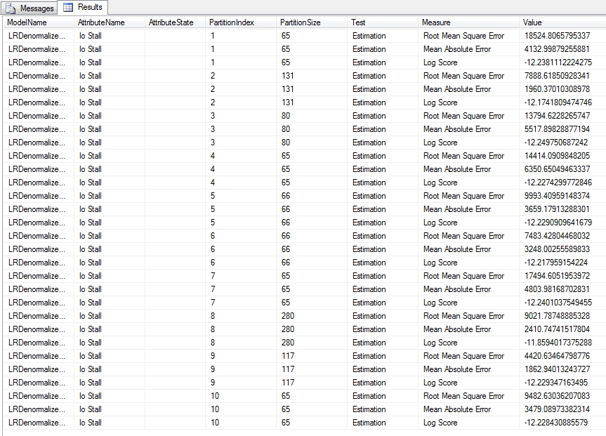
Figure 5 is an example of a Cross-Validation Report for the single Linear Regression model in a mining structure we used earlier in this tutorial series. In the bottom right corner you’ll see figures for the average value for that column in a particular model, as well as the standard deviation, which is a common measure of variability. The higher the value is, the more dissimilar the subsets of the model are from each other. If they vary substantially, that may indicate that your dataset requires more training data.[5] Figure 6 displays part of a lengthy report for one of the DecisionTrees structures we used earlier in this series, which oddly produced sets of values for just two of its five processed models, DTDenormalizedView1ModelDiscrete and DTDenormalizedView1ModelDiscrete2. The results are based on a Target Attribute of “Name” and Target State of “dm_exec_query_stats” (which together refer to the name of a table recorded in the sp_spaceused table we used for practice data) and a Target Threshold of 0.2, Fold Count of 10 and Max Cases of 1,000. In addition to Lift Score, Root Mean Square Error and Log Score we discussed above, you’ll see other measures like True Positive, which refers to the count of successful predictions for the specified attribute-value pair and probability. True Negative refers to cases in which successful predictions were made outside the specified rangers, while False Positive and False Negative refer to incorrect predictions for the same. Explanations for these measures are curiously missing from the current desktop documentation for SQL Server 2012, so your best bet is to consult the MSDN webpage Measures in the Cross-Validation Report for guidance. It also speaks of Pass and Fail measures which are not depicted here, but which refer to assignments of cases to correct and incorrect classifications respectively.
Figure 6: Cross-Validation with Classification and Likelihood Measures (click to enlarge)

Validation for Clustering models is handled a bit differently. In the dropdown list for the Target Attribute you’ll see an additional choice, #CLUSTER, which refers to the cluster number. Selecting this option returns a report like the one depicted below, which contains only measures of likelihood for each cluster. Clustering also uses a different set of DMX stored procedures than the other algorithms to produce the data depicted in cross-validation reports. The syntax for SystemGetClusterCrossValidationResults is the same as the SystemGetCrossValidationResults used by the other algorithms, except that the former does not make use of the Target State and Target Threshold parameters. The same rules that apply in the GUI must also be adhered to in the DMX Code; in Figure 8, for example, we can’t set the Target State or Target Threshold because the predictable attribute we selected has a Content type of Continuous. In both cases, we can add more than one mining model by including it in a comma-separated list. As you can see, the output is equivalent to the cross-validation reports we just discussed.
Figure 7: Cross-Validation with #CLUSTER (click to enlarge)

Figure 8: Cross-Validating a Cluster Using the Underlying DMX Stored Procedure
CALL SystemGetClusterCrossValidationResults(ClusteringDenormalizedView1Structure,ClusteringDenormalizedView1Model, ClusteringDenormalizedView1Model3,
10, — Fold Count
1000 — Max Cases
)

Figure 9: Cross-Validating Using the DMX Stored Procedure SystemGetCrossValidationResults
CALL SystemGetCrossValidationResults(
LRDenormalizedView1Structure, LRDenormalizedView1Model, — more than one model can be specified in a comma-separated list
10, — Fold Count
1000, — Max Cases
‘Io Stall’, — the predictable attribute in this case is Continuous, so we can’t set the Target State and Threshold
NULL, — Target State
NULL) — Target Threshold, i.e. minimum probability, on a scale from 0 to 1

Similarly, we can use other DMX procedures to directly retrieve the measures used to build the scatter plots and lift charts we discussed earlier. As you can see, Figure 10 shows the Root Mean Square Error, Mean Absolute Error and Log Score measures we’d expect when dealing with a Linear Regression algorithm, which is where the data in LRDenormalizedView1Model comes from. The data applies to the whole model though, which explains the absence of a Fold Count parameter. Instead, we must specify a flag that tells the model to use only the training cases, the test cases, both, or either one of these choices with a filter applied as well. In this case we’ve supplied a value of 3 to indicate use of both the training and test cases; see the TechNet webpage “SystemGetAccuracyResults (Analysis Services – Data Mining)” for the other code values. Note that these are the same options we can choose from on the Input Selection tab. I won’t bother to provide a screenshot for SystemGetClusterAccuracyResults, the corresponding stored procedure for Clustering, since the main difference is that it’s merely missing the three attribute parameters at the end of the query in Figure 10.
Figure 10: Using the SystemGetAccuracyResults Procedure to Get Scatter Plot and Lift Chart Data
CALL SystemGetAccuracyResults(
LRDenormalizedView1Structure, LRDenormalizedView1Model, — more than one model can be specified in a comma-separated list
3, — code returning both cases and content from the dataset
‘Io Stall’, — the predictable attribute in this case is Continuous, so we can’t set the Target State and Threshold
NULL, — Target State
NULL) — Target Threshold, i.e. minimum probability, on a scale from 0 to 1

These four stored procedures represent the last DMX code we hadn’t covered yet in this series. It would be child’s play to write procedures like the T-SQL scripts I provided last week to encapsulate the DMX code, so that we can import the results into relational tables. This not only allows us to slice and dice the results with greater ease using views, windowing functions, CASE statements and Multidimensional Expressions (MDX) queries in cubes, but nullifies the need to write any further DMX code, with the exception of prediction queries. There are other programmatic means of accessing SSDM data we have yet to cover, however, which satisfy some narrow use cases and fill some specific niches. In next week’s post, we’ll cover a veritable alphabet soup of additional programming tools like XMLA, SSIS, Reporting Services (RS), AMO and ADOMD.Net which can be used to supply DMX queries to an Analysis Server, or otherwise trigger some kind of functionality we’ve already covered in the GUI.
[1] See the Wikipedia page “Cross Industry Standard Process for Data Mining” at http://en.wikipedia.org/wiki/Cross_Industry_Standard_Process_for_Data_Mining
[2] See the Wikipedia page “SEMMA” at http://en.wikipedia.org/wiki/SEMMA
[3] Yet it is important to keep in mind – as many academic disciplines, which I will not name, have done in recent memory – that this says nothing about how well our dataset might compare with others. No matter how good our sampling methods are, we can never be sure what anomalies might exist in the unknown data beyond our sample. Efforts to go beyond the sampled data are not just erroneous and deceptive, but do disservice to the scientific method by trying to circumvent the whole process of empirical verification. It also defies the ex nihilo principle of logic, i.e. the common sense constraint that you can’t get something for nothing, including information content.
[4] MacLennan, Jamie; Tang, ZhaoHui and Crivat, Bogdan, 2009, Data Mining with Microsoft SQL Server 2008. Wiley Publishing: Indianapolis.
[5] IBID., p. 175.
