A Rickety Stairway to SQL Server Data Mining, Part 11: Model Comparison and Validation

by Steve Bolton               

              Throughout this series of amateur self-tutorials on SQL Server Data Mining (SSDM) I’ve typically included some kind of disclaimer to the effect that I’m writing this in order to learn the material faster (while simultaneously providing the most underrated component of SQL Server some badly needed free press), not because I necessarily know what I’m talking about. This week’s post is proof that I have much more to learn, because I deliberately delayed the important topic of mining model validation until the tail end of the series precisely because I thought it belonged at the end of a typical data mining workflow. A case can still be made for first discussing the nine algorithms Microsoft includes in the product, since we can’t validate mining models we haven’t built yet, but I realized while writing this post that validation can be seen as an initial stage of the process, not merely a coda to assess how well a particular mining project went. I was only familiar with the topic in passing before this post, after having put off formally learning it for several years because of some performance issues which persisted in this week’s experiments, as I’ll get to shortly. For that reason, I never got in the habit of using validation to select the mining models most likely to produce useful information with a minimal investment of server resources. It may be a good idea to perform validation at the end of a project as well, but it ought to be incorporated at earlier stages. In fact, it might be better to view it as one more recurring stage in an iterative mining process. Since data mining is still in its infancy as a field, there may be more of a tendency to view mining projects using the kind of simplistic engineering processes that used to characterize other types of software development, like the old waterfall model. I must confess I unconsciously fell into the trap of assuming simple sequential processes like this without even realizing it, when I should have been applying the Microsoft Solutions Framework formula for software development, which I had to practically memorize back in the day to get pass my last Microsoft Certified Solution Developer (MCSD) certification in Visual Basic 6.0. As I discussed last week, the field has not advanced to the point where it’s standard practice to continually refine the information content of data by mining it recursively, but it will probably come to that someday; scripts like the ones I posted could be used to export mining results back into relational tables, where they can be incorporated into cubes and then mined again. Once refined mining like that become more common, the necessity of performing validation reiteratively at set stages in the circular process will probably be more obvious.
                Until the latest release of SQL Server, validation was always referred to in Microsoft’s documentation as a stage an engineering process called the Cross Industry Standard Process for Data Mining (CRISP-DM). This six-stage process begins with setting the objectives of a project from the perspective of end users plus an initial plan to achieve them, followed by the Data Understanding phase,  in which initial explorations of data are performed with small-scale collections and analysis. Some of the tasks in the Preparation and Modeling phases occur in a circular manner, with continual refinements in data models and collection processes, for example. Validation can be seen as part of the fifth phase, Evaluation, which follows the creation of mining models in the previous phases, in the same order as I’ve deal with these topics in this series. This should lead to the development of models with the highest information content in return for the smallest performance impact, prior to the final phase, Deployment. Elimination of models that don’t perform as expected and substitution with better ones may still be desirable after this point, so validation may be necessary after the deployment phase as well. I have not seen the original documentation for CRISP-DM because their website, crisp-dm.org, has been down for some time, but what I’ve read about it at Wikipedia seems to suggest something of a waterfall model, alongside some recognition that certain tasks would require repetition.[1] Perhaps a more explicit acknowledgment of the iterative nature of the data mining engineering process was slated for inclusion in CRISP-DM 2.0, but this planned revision to the standard is apparently defunct at the moment. The last post at the Cross Industry Standard Process for Data Mining Blog at http://crispdm.wordpress.com/  is titled “CRISP-DM to be Updated” and has a single comment stating that it had been a long time since the status of the project was revised, but rest assured, it was on its way. That was back in 2007. Perhaps CRISP-DM was a victim of its own success, however, because there really hasn’t been any other competing standard since the European Union (EU) got the ball rolling on development of the standard in 1997, with the collaboration of Teradata, NCR, Daimler and two lesser known companies. SEMMA (Sample, Explore, Modify, Model and Assess) is sometimes viewed as a rival to CRISP-DM, but its developer, SAS Institute Inc., says it is  “’rather a logical organization of the functional tool set of’ one of their products, SAS Enterprise Miner.”[2] There are really only so many sane ways to organize a mining project, however, just as there are with other types of software development. It’s not surprising that CRISP-DM has no competition and has had little revision, since it’s fairly self-evident – at least once it’s been thought through for the first time, so credit still must go to its original inventors. Perhaps there is little more that can be done with it, except perhaps to put a little more emphasis on the iterative aspects. This is also the key characteristic of the Microsoft Framework for software development, most of which is entirely applicable to SSDM.
                Until the current version of SQL Server, the MSDN webpage “Validating Data Mining Models (Analysis Services – Data Mining)” said that “CRISP-DM is a well-known methodology that describes the steps in defining, developing, and implementing a data mining project. However, CRISP-DM is a conceptual framework that does not provide specific guidance in how to scope and schedule a project. To better meet the particular needs of business users who are interested in data mining but do not know where to begin planning, and the needs of developers who might be skilled in .NET application development but are new to data mining, Microsoft has developed a method for implementing a data mining project that includes a comprehensive system of evaluation.” This could have been misconstrued to mean that the method of validation employed by Microsoft was proprietary, when in fact it consists of an array of well-known and fairly simple statistical tests, many of which we have already discussed. The same page of documentation, however, does a nice job of summarizing the three goals of validation: 1) ensuring that the model accurately reflects the data it has been fed; 2) testing to see that the findings can be extrapolated to other data, i.e. measures of reliability; and 3) checking to make sure the data is useful, i.e. that it is not riddled with tautologies and other logical problems which might render it true yet meaningless. These goals can sometimes be addressed by comparing a model’s results against other data, yet such data is not always available. Quite often the only recourse is to test a model’s results against the data it has already been supplied with, which is fraught with a real risk of unwittingly investing a lot of resources to devise a really complex tautology. One of the chief means of avoiding this is to divide data into testing and training sets, as we have done throughout this series by leaving the HoldoutSeed, HoldoutMaxPercent and HoldoutMaxCases properties at their default values, which reserves 30 percent of a given model’s data for training. This is an even more important consideration with Logistic Regression and the Neural Network algorithms, which is why they have additional parameters like HOLDOUT_PERCENTAGE, HOLDOUT_SEED and SAMPLE_SIZE that allow users to set similar properties at the level of individual models, not just the parent structures. As detailed in A Rickety Stairway to SQL Server Data Mining, Algorithm 9: Time Series, that mining method handles these matters differently, through the HISTORIC_MODEL_COUNT and HISTORICAL_MODEL_GAP parameters. The former bifurcates a dataset into n number of models, separated by the number of time slices specified in the latter parameter. The built-in validation methods cannot be used with Time Series – try it and you’ll receive the error message “A Mining Accuracy Chart cannot be displayed for a mining model using this algorithm type” – but one of the methods involves testing subsets of a given dataset against each other, as Time Series does in conjunction with the HISTORIC_MODEL_COUNT parameter. By either splitting datasets into testing and training sets or testing subsets against each other, we can use the information content available in a model to test the accuracy of our mining efforts. [3]We can also test mining models based on the same dataset but with different parameters and filters against each other; it is common, for example, to use the Clustering algorithm in conjunction with different CLUSTER_SEED settings, and to pit neural nets with different HOLDOUT_PERCENTAGE, HOLDOUT_SEED and SAMPLE_SIZE values against each other.
               Validation is performed in the last element of the GUI we have yet to discuss, the Mining Accuracy Chart tab, which has four child tabs: Input Selection, Lift Chart, Classification Matrix and Cross Validation. The first of these is used to determine which input is used for the second and is so simple that I won’t bother to provide a screenshot. You merely select as many mining models as you wish from the currently selected structure, pick a single column common to all of them and optionally, select a single value for that column to check for. Then you either select one of the three radio buttons labeled Use mining model test cases, Use mining structure test cases and Specify a different data set. The last of these options brings up the window depicted in Figure 1, which you can use to choose a different external dataset from a separate mining structure or data source view (DSV) to test the current dataset against. You must supply column mappings there, in the same manner as on the Mining Model Prediction tab we discussed two posts ago in A Rickety Stairway to SQL Server Data Mining, Part 10.3: DMX Prediction Queries. The third radio button also enables a box to input a filter expression. You’ll also notice a checkbox labeled Synchronize prediction columns and values at the top of the tab, which Books Online (BOL) says should normally remain checked; this is not an option I’ve used before, but I assume from the wording of the documentation that this is a rare use case when mining models within the same structure have a column with the same name, but with different values or data types. The only difficulty I’ve had thus far with this tab is the Predict Value column, which I’ve been unable to type any values into and has not been automatically populated from the data of any model I’ve validated yet.

Figure 1: Specifying a Different Data Set in the Input Selection Tab

                The Input Selection tab doesn’t present any data; it merely specifies what data to work with in the Lift Chart tab. The tab will automatically display a scatter plot if you’re working with a regression (which typically signifies a Content type of Continuous) or a lift chart if you’re not. We’ve already briefly touched upon scatter plots and the concept of statistical lift earlier in this series, but they’re fairly simple and serve similar purposes. In the former, a 45 degree line in the center represents the ideal prediction, while the rest of the graph is filled with data points in which predicted values run along the vertical axis and the actual values on the horizontal axis. You can also hover over a particular data point to view the predicted and actual values that specify its location. The closer the data points are in a scatter plot, the better the prediction. It’s really a fairly simple idea, one that is commonly introduced to high school and early college math students. Generating the scatter plot is easier said than done, however, because I have seen the Visual Studio devenv.exe run on one core for quite a while on these, followed by the SQL Server Analysis Services (SSAS) process msmdsrv.exe as also running on a single core and consuming more than a gigabyte of RAM, before crashing Visual Studio altogether on datasets of moderate size. This is the first performance pitfall we need to be wary of with validation, although the results are fairly easy to interpret if the process completes successfully. As depicted in Figure 2,  the only complicated part about this type of scatter plot with SSDM validation is that you may be seeing data points from different models displayed in the same chart, which necessitates the use of color coding. In this case we’re looking at data for the CpuTicks column in the mining models in the ClusteringDenormalizedView1Structure, which we used for practice data in A Rickety Stairway to SQL Server Data Mining, Algorithm 7: Clustering. The scores are equivalent to the Score Gain values in the NODE_DISTRIBUTION tables of the various regression algorithms we’ve covered to date; these represent the Interestingness Score of the attribute, in which higher numbers represent greater information gain, which is calculated by measuring the entropy when compared against a random distribution.

Figure 2: Multiple Mining Models in a Scatter Plot

 
              The object with scatter plots is to get the data points as close to the 45-degree line as possible, because this indicates an ideal regression line. As depicted in Figure 3, Lift charts also feature a 45-degree line, but the object is to get the accompanying squiggly lines representing the actual values to the top of the chart as quickly as possible, between the random diagonal and the solid lines representing hypothetical perfect predictions. Users can easily visualize how much information they’ve gained through the data mining process with lift charts, since it’s equivalent to the space between the shaky lines for actual values and the solid diagonal. The really interesting feature users might overlook at first glance, however, is that lift charts also tell you how many cases must be mined in order to return a given increase in information gain. This is represented by the grey line in Figure 3, which can be set via the mouse to different positions on the horizontal axis, in order to specify different percentages of the total cases. This lift chart tells us how much information we gained for all values of CounterID (representing various SQL Server performance counters, from the IO data used for practice purposes earlier in the series) for the DTDenormalizedView1Structure mining structure we used in A Rickety Stairway to SQL Server Data Mining, Algorithm 3: Decision Trees. If I had been able to type in the Predict Value column in the Input Selection box, I could have narrowed it down to just a single specific value for the column I chose, but as mentioned before, I have had trouble using the GUI for this function. Even without this functionality, we can still learn a lot from the Mining Legend, which tells us that with 18 percent of the cases – which is the point where the adjustable grey line crosses the diagonal representing a random distribution – we can achieve a lift score of 0.97 on 77.11 percent of the target cases for one mining model, with a probability of 35.52 percent of meeting the predicted value for those cases. The second model only has a lift score of 0.74 for 32.34 percent of the cases with a probability of 25.84 at the same point, so it doesn’t predict as well by any measure. As BOL points out, you may have to balance the pros and cons of using a model with higher support coverage and a lower probability against models that have the reverse. I didn’t encounter that situation in any of the mining structures I successfully validated, in all likelihood because the practice data I used throughout this series had few Discrete or Discretized predictable attributes, which are the only Content types lift charts can be used with.

Figure 3: Example of a Lift Chart (click to enlarge)

                Ideally, we would want to predict all of the cases in a model successfully with 100 percent accuracy, by mining as few cases as possible. The horizontal axis and the grey line that identifies an intersection along it thus allow us to economize our computational resources. By its very nature, it also lends itself to economic interpretations in a stricter sense, since it can tell us how much investment is likely to be required in order to successfully reach a certain percentage of market share. Many of the tutorials I’ve run across with SSDM, particularly BOL and Data Mining with Microsoft SQL Server 2008,the classic reference by former members of Microsoft’s Data Mining Team[4], use direct mailing campaigns as the ideal illustration for the concept. It can also be translated into financial terms so easily that Microsoft allows you to transform the data into a Profit Chart, which can be selected from a dropdown control. It is essentially a convenience that calculates profit figures for you, based on the fixed cost, individual cost and revenue per individual you supply for a specified target case size, then substitutes this more complex statistic for the target case figure on the x-axis. We’re speaking of dollars and people instead of cases, but the Profit Chart represents the same sort of relationships: by choosing a setting for the percentage of total cases on the horizontal axis, we can see where the grey line intersects the lines for the various mining models to see how much profit is projected. A few more calculations are necessary, but it is nothing the average college freshman can’t follow. In return, however, Profit Charts provide decision makers with a lot of power.
              Anyone who can grasp profit charts will find the classification matrices on the third Mining Accuracy Chart tab a breeze to interpret. First of all, they don’t apply to Continuous attributes, which eliminated most of my practice data from consideration; this limitation may simplify your validation efforts on real world data for the same reason, but it of course comes at the cost of returning less information your organization’s decision makers could act on. I had to hunt through the IO practice data we used earlier in this series to find some Discrete predictable attributes with sufficient data to illustrate all of the capabilities of a Classification Matrix, which might normally have many more values listed than the three counts for the two mining models depicted below. The simplicity of the example makes it easier to explain the top chart in Figure 1, which can be read out loud like so: “When the mining model predicted a FileID of 3, the actual value was correct in 1,147 instances and was equal to FileID #1 or #2 in 0 instances. When it predicted a FileID of 1, it was correct 20,688 times and made 116 incorrect predictions in which the actual value was 2. When the model predicted a FileID of 2, it was correct 20,607 times and made 66 incorrect predictions in which the actual value turned out to be 1.” The second chart below is for the same column on a different model in the same structure, in which a filter of Database Id = 1 was applied

Figure 4: A Simple Classification Matrix

                 The Cross Validation tab is a far more useful tool – so much so that it is only available in Enterprise Edition, so keep that in mind when deciding which version of SQL Server your organization needs to invest in before starting your mining projects. The inputs are fairly easy to explain: the Fold Count represents the number of subsets you want to divide your mining structure’s data into, while the Target Attribute and Target State let you narrow the focus down to a particular attribute or attribute-value pair. Supplying a Target State with a Continuous column will elicit the error message “An attribute state cannot be specified in the procedure call because the target attribute is continuous,” but if a value is supplied with other Content types then you can also specify a minimum probability in the Target Threshold box. I strongly recommend setting the Max Cases parameter when validating structures for the first time, since cross-validation can be resource-intensive, to the point of crashing SSAS and Visual Studio if you’re not careful. Keeping a Profiler trace going at all times during development may not make the official Best Practices list, but it can definitely be classified as a good idea when working with SSAS. It is even truer with SSDM and truer still with SSDM validation. This is how I spotted an infinitely recursive error labeled “Training the subnet. Holdout error = -1.#IND00e+000” that began just four cases into my attempts to validate one of my neural net mining structures. The validation commands kept executing indefinitely even after the Cancel command in Visual Studio had apparently completed. I haven’t yet tracked down the specific cause of this error, which fits the pattern of other bugs I’ve seen that crash Analysis Services through infinite loops involving indeterminate (#IND) or NaN values. Checking the msmdsrv .log revealed a separate series of messages like, “An error occurred while writing a trace event to the rowset…Type: 3, Category: 289, Event ID: 0xC121000C).” On other occasions, validation consumed significant server resources – which isn’t surprising, given that it’s basically doing a half-hearted processing job on every model in a mining structure. For example, while validating one of my simpler Clustering structures with just a thousand cases, my beat-up development machine ran on just one of six cores for seven and a half minutes while consuming a little over a gigabyte of RAM. I also had some trouble getting my Decision Trees structures to validate properly without consuming inordinate resources.
               The information returned may be well worth your investment of computational power though. The information returned in the Cross-Validation Report takes a bit more interpreting because there’s no eye candy, but we’re basically getting many of the figures that go into the fancy diagrams we see on other tabs. All of the statistical measures it includes are only one level of abstraction above what college freshmen and sophomores are exposed to in their math prereqs and are fairly common, to the point that we’ve already touched on them all throughout this series. For Discrete attributes, lift scores like the ones we discussed above are calculated by dividing the actual probabilities by the marginal probabilities of test cases, with Missing values left out, according to BOL. Continuous attributes also have a Mean Absolute Error which indicates greater accuracy inversely, by how small the error is. Both types are accompanied by a Root Mean Square Error, which is a common statistical tool calculated in this case as the “square root of the mean error for all partition cases, divided by the number of cases in the partition, excluding rows that have missing values for the target attribute.” Both also include a Log Score, which is only a logarithm of the probability of a case. As I have tried to stress throughout this series, it is far more important to think about what statistics like these are used for, not the formulas they are calculated by, for the same reason that you really ought not think about the fundamentals of internal combustion engines while taking your driver’s license test. It is better to let professional statisticians who know that topic better than we do worry about what going on under the hood; just worry about what the simpler indicators like the speedometer are telling you. The indicators we’re working with here are even simpler, in that we don’t need to worry about them backfiring on us if they get too high or too low. In this instance, minimizing the Mean Absolute Error and Root Mean Square Error and maximizing the Lift Score are good; the opposite is bad. Likewise, we want to maximize the Log Score because that means better predictions are more probable. The logarithm part of it only has to do with converting the values returned to a scale that is easier to interpret; the calculations are fairly easy to learn, but I’ll leave them out for simplicity’s sake. If you’re a DBA, keep in mind that mathematicians refer to this as normalizing values, but it really has nothing in common with the kind of normalization we perform in relational database theory.                                                                                                                                                                          

Figure 5: Cross-Validation with Estimation Measures (click to enlarge)

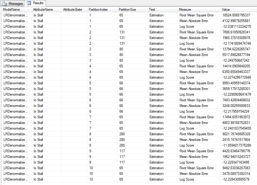
                Figure 5 is an example of a Cross-Validation Report for the single Linear Regression model in a mining structure we used earlier in this tutorial series. In the bottom right corner you’ll see figures for the average value for that column in a particular model, as well as the standard deviation, which is a common measure of variability. The higher the value is, the more dissimilar the subsets of the model are from each other. If they vary substantially, that may indicate that your dataset requires more training data.[5] Figure 6 displays part of a lengthy report for one of the DecisionTrees structures we used earlier in this series, which oddly produced sets of values for just two of its five processed models, DTDenormalizedView1ModelDiscrete and DTDenormalizedView1ModelDiscrete2. The results are based on a Target Attribute of “Name” and Target State of “dm_exec_query_stats” (which together refer to the name of a table recorded in the sp_spaceused table we used for practice data) and a Target Threshold of 0.2, Fold Count of 10 and Max Cases of 1,000. In addition to Lift Score, Root Mean Square Error and Log Score we discussed above, you’ll see other measures like True Positive, which refers to the count of successful predictions for the specified attribute-value pair and probability. True Negative refers to cases in which successful predictions were made outside the specified rangers, while False Positive and False Negative refer to incorrect predictions for the same.  Explanations for these measures are curiously missing from the current desktop documentation for SQL Server 2012, so your best bet is to consult the MSDN webpage Measures in the Cross-Validation Report for guidance. It also speaks of Pass and Fail measures which are not depicted here, but which refer to assignments of cases to correct and incorrect classifications respectively.

Figure 6: Cross-Validation with Classification and Likelihood Measures (click to enlarge)

               Validation for Clustering models is handled a bit differently. In the dropdown list for the Target Attribute you’ll see an additional choice, #CLUSTER, which refers to the cluster number. Selecting this option returns a report like the one depicted below, which contains only measures of likelihood for each cluster. Clustering also uses a different set of DMX stored procedures than the other algorithms to produce the data depicted in cross-validation reports. The syntax for SystemGetClusterCrossValidationResults is the same as the SystemGetCrossValidationResults used by the other algorithms, except that the former does not make use of the Target State and Target Threshold parameters. The same rules that apply in the GUI must also be adhered to in the DMX Code; in Figure 8, for example, we can’t set the Target State or Target Threshold because the predictable attribute we selected has a Content type of Continuous. In both cases, we can add more than one mining model by including it in a comma-separated list. As you can see, the output is equivalent to the cross-validation reports we just discussed.

Figure 7: Cross-Validation with #CLUSTER (click to enlarge)

Figure 8: Cross-Validating a Cluster Using the Underlying DMX Stored Procedure
CALL SystemGetClusterCrossValidationResults(ClusteringDenormalizedView1Structure,ClusteringDenormalizedView1Model, ClusteringDenormalizedView1Model3,
10, — Fold Count
1000 — Max Cases
)

 

Figure 9: Cross-Validating Using the DMX Stored Procedure SystemGetCrossValidationResults
CALL SystemGetCrossValidationResults(
LRDenormalizedView1Structure, LRDenormalizedView1Model, — more than one model can be specified in a comma-separated list
10, — Fold Count
1000, — Max Cases
‘Io Stall’, — the predictable attribute in this case is Continuous, so we can’t set the Target State and Threshold
NULL, — Target State
NULL) — Target Threshold, i.e. minimum probability, on a scale from 0 to 1

 

               Similarly, we can use other DMX procedures to directly retrieve the measures used to build the scatter plots and lift charts we discussed earlier. As you can see, Figure 10 shows the Root Mean Square Error, Mean Absolute Error and Log Score measures we’d expect when dealing with a Linear Regression algorithm, which is where the data in LRDenormalizedView1Model comes from. The data applies to the whole model though, which explains the absence of a Fold Count parameter.  Instead, we must specify a flag that tells the model to use only the training cases, the test cases, both, or either one of these choices with a filter applied as well. In this case we’ve supplied a value of 3 to indicate use of both the training and test cases; see the TechNet webpage “SystemGetAccuracyResults (Analysis Services – Data Mining)” for the other code values. Note that these are the same options we can choose from on the Input Selection tab. I won’t bother to provide a screenshot for SystemGetClusterAccuracyResults, the corresponding stored procedure for Clustering, since the main difference is that it’s merely missing the three attribute parameters at the end of the query in Figure 10.

Figure 10: Using the SystemGetAccuracyResults Procedure to Get Scatter Plot and Lift Chart Data 
CALL SystemGetAccuracyResults(
LRDenormalizedView1Structure, LRDenormalizedView1Model, — more than one model can be specified in a comma-separated list
3, — code returning both cases and content from the dataset
‘Io Stall’, — the predictable attribute in this case is Continuous, so we can’t set the Target State and Threshold
NULL, — Target State
NULL) — Target Threshold, i.e. minimum probability, on a scale from 0 to 1

 

               These four stored procedures represent the last DMX code we hadn’t covered yet in this series. It would be child’s play to write procedures like the T-SQL scripts I provided last week to encapsulate the DMX code, so that we can import the results into relational tables. This not only allows us to slice and dice the results with greater ease using views, windowing functions, CASE statements and Multidimensional Expressions (MDX) queries in cubes, but nullifies the need to write any further DMX code, with the exception of prediction queries. There are other programmatic means of accessing SSDM data we have yet to cover, however, which satisfy some narrow use cases and fill some specific niches. In next week’s post, we’ll cover a veritable alphabet soup of additional programming tools like XMLA, SSIS, Reporting Services (RS), AMO and ADOMD.Net which can be used to supply DMX queries to an Analysis Server, or otherwise trigger some kind of functionality we’ve already covered in the GUI.

---

[1] See the Wikipedia page “Cross Industry Standard Process for Data Mining” at http://en.wikipedia.org/wiki/Cross_Industry_Standard_Process_for_Data_Mining

[2] See the Wikipedia page “SEMMA” at http://en.wikipedia.org/wiki/SEMMA

[3] Yet it is important to keep in mind – as many academic disciplines, which I will not name, have done in recent memory – that this says nothing about how well our dataset might compare with others. No matter how good our sampling methods are, we can never be sure what anomalies might exist in the unknown data beyond our sample. Efforts to go beyond the sampled data are not just erroneous and deceptive, but do disservice to the scientific method by trying to circumvent the whole process of empirical verification. It also defies the ex nihilo principle of logic, i.e. the common sense constraint that you can’t get something for nothing, including information content.

[4] MacLennan, Jamie; Tang, ZhaoHui and Crivat, Bogdan, 2009, Data Mining with Microsoft SQL Server 2008. Wiley Publishing: Indianapolis.

[5] IBID., p. 175.

A Rickety Stairway to SQL Server Data Mining, Part 10.4: Data Mining Dimensions vs. Drastic Dynamic DMX

by Steve Bolton

                Anyone who’s gotten this far in this series of amateur self-tutorials on SQL Server Data Mining (SSDM) is probably capable of using it to unearth some worthwhile nuggets of wisdom in their data. One of the key remaining questions at this step of our rickety stairway is what we can do with the information we’ve mined. The most obvious answer to this would be to act upon the information; we must not lose sight of the fact that our ultimate mission is not to simply dig up truths based on past data for a person or organization, but to enable them to act with greater precision in the present to ensure a better future. Any subject under the sun may an intrinsic worth of its own, but appreciation for anything should not be divorced from its wider uses and implications for everything else beyond it; this is the point at which intellectuals to get lost in Ivory Towers and become irrelevant to the wider world outside their narrow vision. This also happens in the discipline of history, which I have some claim to real expertise in – unlike with SSDM, which I am writing about in order to familiarize myself with the topic better while simultaneously giving SQL Server’s most neglected component some badly needed free press. Sometimes historians get lost in mere antiquarian appreciation for their narrow specialties, while ignoring the more important tasks of helping mankind avoid fulfilling Santayana’s classic warning, “Those who cannot remember the past are condemned to repeat it.” Likewise, as the field of data mining blossoms in the coming decades, it will be critical to keep the giant mass of truths it is capable of unearthing relevant to the goals of the organizations the miners work for. Knowledge is worth something on its own, but it should also be remembered that “Knowledge is power.” Francis Bacon’s famous quip is incomplete, however, because knowledge is only one form of power; as Stephen King once pointed out in typically morbid fashion, it doesn’t do a mechanic whose car jack has slipped much good to truly know that he’s powerless to move the automobile crushing his chest. I suspect this is a fine distinction that will come to the fore as data mining matures. The most critical bottlenecks for organizations in the future, once data mining has become ubiquitous, may be the challenge of acting on it. The poor soul in Stephen King’s example can’t act on his information at all. Many organizations, however, may prove incapable of acting on good data due to other internal faults. Eight centuries ago, St. Thomas Aquinas pointed out that sometimes people prove incapable of doing things they know they ought to do, despite telling themselves to do them; such “defects of command” may well become glaringly evident in the future, as the next bottlenecks in unsuccessful organizations.
                At that point, data mining may already be automated to the point where algorithm processing results mechanically trigger actions by organizations. Some relational databases and data warehouses already have the capability of doing this to a degree, such as automatically sending out new orders to replenish inventories before they are depleted, or triggering a stock trade. Yet in most cases these automated decisions are based on fairly simple functions, not the ultra-, uber-, mega-sophisticated functions that modern data mining algorithms amount to. One day Wall Street firms may rise and fall in a day depending on whether the gigantic data warehouse at the center of an organization can out-mine its competitors and therefore out-trade them, without any human intervention at all since the formulas they’re acting on are too complex to put into human language; this would be a strange twist indeed on the science fiction chestnut of artificial intelligence gone awry. Using some of the scripts I’m going to provide in this post in conjunction with ADO.Net, SQL Server Integration Services (SSIS) and XML for Analysis (XMLA), we could indeed start laying the foundations for such automated processes right now, if need be.  The problem is that data mining is still in its infancy, to the point where it would be quite unwise for any organization to automatically rely on its mining results without prior human review by an actual intelligence. Our next programming task could thus be to build systems that automatically act on data mining results, but for the meantime it is much more prudent for humans to review the results first, then decide on courses of action themselves. That is probably why SSDM, or any other mining software I’m aware of, lacks built-in ways of handling such functionality. Without it, programmers are left with two other tasks they can perform on data they’ve already mined: present it more efficiently so that people can analyze it from a human perspective, or to feed the data back into mining process for further computational analysis. Either way, we’re talking about mining the mining results themselves; the process can be looked at as continuously refining hydrocarbon fuels or cutting diamonds we’ve taken from the ground, until they reach the point where the cost of further refining outweighs further improvements in quality. To perform the latter task, we need some programmatic means of feeding mining results from SSDM back into the mining process. Keep in mind that this is a fairly advanced task; it is obviously much more important to mine data the first time, as the previous posts in this series explained how to do, than to feed them back into the system reiteratively. It is not as advanced or risky as automated action though. That is probably why some limited means to perform the former task are provided in SSDM, but not any out-of-the-box solutions to the latter one.
               Such nascent functionality is included in SSDM in the form of data mining dimensions, which incorporate your mining results into a SQL Server Analysis Services (SSAS) cube. The official documentation carries a caveat that makes all the difference in the world: “If your mining structure is based on an OLAP cube.” The practice data I used throughout this series came strictly from relational data, because I didn’t want to burden DBAs who come from a relational background with the extra step of first importing our data into a cube, then into SSDM. That is why I was unable to add a data mining dimension through the usual means of right-clicking on a mining model and selecting the appropriate menu item, as depicted in Figure 1. I discovered this important limitation after getting back just 34 hits for the Google search terms “’Create Data Mining Dimension’ greyed” (or grayed) – all of which led to the same thread at MSDN with no reply.

Figure 1: Mining Dimension Creation Menu Command

                The rest of the screenshots in this post come from another project I started practicing on a long time ago, which was derived from cube data and therefore left the Create a Data Mining Dimension command enabled. Selecting it brings up the dialog in Figure 2, which performs the same function as the Create mining model dimension checkbox and a Create cube using mining model dimension checkbox on the Completing the Wizard page of the Data Mining Wizard. It’s all fairly self-explanatory.

Figure 2: Mining Dimension Creation Dialog Box

                A new data source view (DSV) is added to your project after you create the mining dimension. Depending on the algorithm you’ve chosen, certain columns from SSDM’s common metadata format will be automatically added to a MiningDimensionContentNodes hierarchy, including ATTRIBUTE_NAME, NODE_RULE, NODE_SUPPORT and NODE_UNIQUE_NAME. Some of these columns may be entirely blank and even those that are not provide only a fraction of the numeric data the algorithms churn out, such as NODE_SUPPORT, which is a mere case count. Such miserly returns would hardly be worth the effort unless we add more numeric columns for SSAS to operate on, such as NODE_PROBABILITY and MSOLAP_NODE_SCORE from the DSV list on the right-hand side of Figure:

Figure 3: Available Mining Dimension Columns

                Even after including these columns, you may not see any worthwhile data depicted in the cube’s Browser tab till you right-click the white space in the table and check the Include Empty Cells command, as depicted in Figure 4.

Figure 4: Include Empty Cells

                Data mining dimensions are of limited use in their current form, however, because of a welter of serious inadequacies. As mentioned before, your data will have to be imported from a cube instead of a relational database, but it can also only be exported to a cube, not into a relational table; even within SSAS, you’re limited to incorporating it is a dimension, not a fact table. Furthermore, they only work with four of SQL Server’s nine data mining algorithms, Decision Trees, Clustering, Sequence Clustering and Association Rules, so we’re crippled right off the bat. One of these is narrowly specialized, as discussed in A Rickety Stairway to SQL Server Data Mining, Algorithm 8: Sequence Clustering, and another is a brute force algorithm that is high popular but appropriate only in a narrow set of use cases, as explained in A Rickety Stairway to SQL Server Data Mining, Algorithm 6: Association Rules. Furthermore, the data provided in mining dimensions comes solely from the common metadata format I introduced in A Rickety Stairway to SQL Server Data Mining, Part 0.1: Data In, Data Out. As I reiterated in each individual article on the nine algorithms, the format is capable of holding apples and oranges simultaneously (like a produce stand), but it comes at the cost of a bird’s nest of nested tables and columns which change their meaning from one algorithm to the next, or even one row to the next depending on the value of such flags as NODE_TYPE and VALUETYPE. The first instinct of anyone who comes from a relational background is to normalize it all, not necessarily for performance reasons, but for logical clarity. If you’re among this crowd, then you’re in luck, because the scripts I’m providing here will allow you to follow those instincts and import all of your mining results into relational tables.
                The concept is really quite simple, at least initially: you create a linked server to your SSAS database using sp_addlinkedserver or the GUI in SQL Server Management Studio (SSMS), then issue DMX queries through OpenQuery. For explicit directions, see the SQLServerDataMining.com webpage Getting Data Mining Results into SQL Tables posted by the user DMTeam on Oct. 24, 2008, but there’s not much left to say about that end of it.[i] The difficult part is formatting your DMX correctly, which can be challenging enough in an SSMS DMX Query window. There are many idiosyncrasies to the language which take getting used to, such as the odd necessity of putting brackets around the PARENT_UNIQUE_NAME column in all situations, the difficulty of scoping FLATTENED columns from NODE_DISTRIBUTION tables and a dozen others. One of the most nagging limitations is the inability of SQL Server to import its own SSDM results using the standard Microsoft OLE DB for Analysis Services data provider, which crashes whenever #IND (indeterminate) or NaN values are encountered in the mined data. The workaround I’ve developed currently requires you to have a copy of Microsoft Excel on your SSAS server because it uses Excel functions to format the #IND and NaN values correctly, but I will probably post a better solution that doesn’t require Excel fairly soon, now that I know how to write SSAS stored procedures. This can be a nightmare to debug, but the scripts I’ll provide take care of the problem for you. Debugging DMX in its native environment is difficult enough, but trying to track down a single error in a query that’s twenty lines long can be a mind-numbing experience when it’s nested inside a T-SQL OpenQuery statement. For all intents and purposes, you’re then also dealing with tracking endless quote marks just as you would with dynamic SQL. If you want to persist the results you’re going to have to use either sp_executesql or INSERT EXEC to get them into a temporary table, thereby adding another layer of quote marks to keep track of.
                The scripts I’m providing here relieve you of most of this burden of coding your own DMX, with the exception of prediction queries. These are handled by the PredictionQuerySP stored procedure I’ve also incorporated, which allows you to execute your own DMX queries in T-SQL, including those with functions that require quote marks, by doubling them like so: EXEC Mining.PredictionQuerySP‘MonitoringLS’, ‘SELECT ClusterProbability(”Cluster 1”) FROM [ClusteredDenormalizedView1Model2]’. This code can be downloaded here, along with the other stored procedures for importing DMX data into T-SQL. The code was designed with SSMS T-SQL queries in mind, but it can be easily updated to accommodate queries submitted from other data access tools that don’t require double quoting, by adding a simple bit flag and IF statement. Aside from prediction queries, you need not write your own DMX at all, since the eight ImportContent stored procedures (two of the nine algorithms, Logistic Regression and neural nets, share the same procedure and table structure) I’m providing here encapsulate the whole process of transferring your mining results directly into the relational tables created by the companion Data Definition Language (DDL) scripts. There are also procedures and corresponding tables to import any information DMX queries can provide about mining structures, models, their columns and parameters. The procedures also take care of the messy work of normalizing all of SSDM’s nested tables into hierarchies of relational tables. I came up with this solution just a few weeks ago, after I tried to resuscitate a bunch of ad hoc scripts I’d written over the years for this article, only to realize that a more comprehensive and integrated architecture would make more sense. That left me no time to incorporate the necessary error checking or transactions in the procedures, add appropriate nonclustered indexes on the tables, try performance tuning, or any other such considerations. Don’t depend on these scripts until you’ve verified the accuracy of their results first. There are guaranteed to be mistakes in the code, which is a hodgepodge of dynamic SQL, CTEs, MERGE statements and multiple instances of a workaround I developed for the silly limitations Microsoft put on nested INSERT EXEC statements. Feel free to update it to your liking; just please give me credit when possible, because I’d like to get paid at some point for investing all of this energy learning yet another field. I intend to upgrade the scripts on my own for the purely selfish reason that they will help save me the time of writing any more DMX, except in the case of prediction queries. If there’s sufficient interest, I’ll post my revisions here. There’s no reason why we have to reinvent the wheel with each DMX query, when we can write all we need in one big guzzle like this, then store it in a single standardized, interchangeable format. The DDL statements to create the schema in Figure 5 are available here.

Figure 5: Schema v. 0.1 for Importing DMX into Relational Tables (click to enlarge)

                Your first task in importing SSDM results into this relational schema is to start at the top of the object model and create a new row for your SSAS database in the Mining.SSASDatabase; I haven’t created a stored procedure for this yet, because the metadata for this table is not yet set, so its really only useful at this point for generating identity foreign keys for the MiningStructureTable column SSASDatabaseID. Then use Mining.ImportStructureTableSP to create or update your list of mining structures, by supplying the procedure with the linked server and SSAS database names. At present I haven’t added code to simplify the process any further, so you’ll have to use the identity value generated for a particular structure when running Mining.ImportColumnTableSP and Mining.ImportModelTableSP, which gets the column information and collection of mining models in a single structure. The latter procedure also records the algorithm settings for a particular model, but the model column information will have to be retrieved by supplying the model identity value auto-generated by Mining.ImportModelTableSP to Mining.Import.ModelColumnTableSP. Once these steps are complete, you can import all of your model’s processing results into the appropriate table type, by choosing from one of the following stored procedures based on the model’s selected algorithm: ImportAssociationRulesModelContentSP, ImportClusterModelContentSP, ImportDecisionTreesModelContentSP, ImportLinearRegressionModelContentSP, ImportNaiveBayesModelContentSP, ImportNNModelContentSP and ImportTimeSeriesModelContentSP. They all take an identical set of parameters, including the linked server name, database name and model identity value, like so: EXEC [Mining].[ImportLinearRegressionModelContentSP]‘MonitoringLS‘, ‘MonitorMiningProject’, 18.
                What you can you do with the data once it’s been imported into relational tables? The sky’s the limit. You could create customized views of the results and apply fine-grained security access rights to them; perform sophisticated ANOVA analyses of your mining results; do custom clustering operations; slice and dice the data with the exciting new T-SQL windowing functions; or even build views to compare the intercepts of your regressions across models, or models applying different algorithms, should that prove meaningful to you. Best of all, you can then feed the data into the fact tables and dimensions of an SSAS cube – including the NODE_DISTRIBUTION table data, which you can’t extract through ordinary data mining dimensions – then mine the results again. You could conceivably continue this process recursively, if you had the need and the computational resources. As I explained in A Rickety Stairway to SQL Server Data Mining, Part 0.1: Data In, Data Out, data mining algorithms consist of combinations of statistical building blocks, which could conceivably be arranged in an infinite array of permutations. This whole series is predicated on the idea that a person without a doctorate in statistics can still use these algorithms and their building blocks without understanding their inner workings, as long as they grasp their uses – just as a driver only needs to know what a brake and steering wheel do, not how to reverse engineer them. Therefore I can’t predict what combinations of statistical building blocks you may find useful for a particular project, only that incorporating the results into relational tables will give you much greater freedom to apply them as you see fit.
              SSDM is impressive, but you reach the limits of what you can do with the data once you include it in a data mining dimension or depict it in the GUI; by importing the data into other tools, you can not only present the results differently, but perform further analysis. In my next post, we’ll make mention of four DMX stored procedures we have yet to cover, since they’re advanced means of performing validation tasks on mining models. After that we’ll get into ADO.Net, SSIS tasks, XMLA, Reporting Services and other such alternative means of accessing and extending SSDM programmatically. Functionally, writing custom code and model validation ought to come after learning how to use the nine algorithms correctly, since we can’t validate or retrieve what hasn’t yet been processed. Writing DMX and accessing SSDM with tools like SSIS is not an absolute necessity though, because users can always depend on the GUI tools to view their mining results, as explained in previous posts. It is less practical to do without model validation though, since this is a critical step in the mining process. Why should we rely on the results of faulty models and waste further server resources on them, when statistical and programmatic means are already available to us that can tell us if they’re defective? Stay tuned for that essential step up this long stairway. After that point we will be up the ladder to the roof and practically doing cartwheels on the chimney, which will be the ideal point for a final tutorial or two to close out the series, on the arcane topics of Predictive Model Markup Language (PMML) and plug-in algorithms.

---

[i] In previous iterations I depended on nearly identical information provided by other posters and sites, which I neglected to keep records of, so I can’t properly cite them. There isn’t much room for creativity with the basic formula they all provide for importing DMX queries so a citation probably isn’t necessary – yet I like to cover all my bases, so I found that citation at SQLServerDataMining before using it to overhaul these scripts a few weeks back.

A Rickety Stairway to SQL Server Data Mining, Part 10.3: DMX Prediction Queries

 
by Steve Bolton

               In the last two installments of this series of amateur self-tutorials on SQL Server Data Mining (SSDM), I discussed how to performed Data Definition Language (DDL) and Data Manipulation Language (DML) tasks with Data Mining Expressions (DMX), the SQL-like language used to administer SSDM. These topics were easier to explain and less critical to know than the material covered in previous posts, like the installments on SSDM’s nine algorithms; furthermore, the syntax for both operations is far simpler and serves far fewer purposes than DDL and DML with T-SQL and Multidimensional Expressions (MDX), the languages used for relational tables and OLAP cubes in SQL Server. Much of the functionality DMX provides can be also be performed faster in the GUI of SQL Server Data Tools (SSDT) and is thus only useful in certain limited scenarios. This is less true, however, of prediction queries, which allow users to make calculations based on the patterns contained in a previously trained mining model, sometimes by feeding it sets of input values that don’t exist in the model. It is often more difficult or even impossible to perform the same tasks without writing DMX code, which makes prediction queries the most important component of the language. We can perform some of the same tasks using the Mining Model Prediction tab in SSDT, which isn’t difficult to understand if you’ve already used the tools in SSDT and Visual Studio provides to graphically create tables and views instead of coding them by hand with T-SQL. Figure 2 is a screenshot of the tab, in which a few columns of the LRDenormalizedView1Model mining model we used previously in this series are selected in the table to the left and then appear in the grid at the bottom; to see the predicted values when compared against the set of cases selected to the right, simply right-click the tab surface and select the Result menu item. To view the DMX query the tool uses to create the prediction, select Query. The rest is fairly self-explanatory, except for the Singleton Query menu item, which requires an introduction to the various types of DMX prediction queries. Like equivalent graphical tools that generate T-SQL to create tables and views, the Mining Model Prediction Tab is awkward and deceptively simplistic; it seems like it ought to save you the trouble of writing DMX code, but often does not. As discussed in previous posts, the use cases for DML and DDL in DMX are quite limited because many of the same tasks can be performed more efficiently through the GUI, but prediction queries (like stored procedures and views in T-SQL) are really the one part of DMX that can typically be more efficiently coded by hand.

Figure 1: The Mining Model Prediction Tab

                The equivalent functionality in DMX is provided by a couple of interdependent clauses and functions which are often used in concert. The first of these are prediction joins, which employs syntax elements similar to those of T-SQL joins to compare the patterns stored in a mining model against a set, which can come from explicitly defined valued, the results of a sub-select, an MDX query or the data returned by an OpenQuery statement. To test a particular case (i.e., a single row of values) against your model, you supply a FROM statement coupled with the mining model name, followed by a PREDICTION JOIN clause with a list of explicit hand-coded values corresponding to the columns in the model. An example of such a “singleton query” can be found in Figure 4, in which we see what output is returned from a mining model we used in A Rickety Stairway to SQL Server Data Mining, Algorithm 5: The Neural Network Algorithm, when it is supplied with specific values for the DatabaseID and FileHandleID columns. In that query I used the NATURAL PREDICTION JOIN clause, which automatically correlates the columns from the mining model and the joined set together based on their names. If the keyword NATURAL is left out, then you must manually correlate each set of columns together using ON clauses in much the same manner as in a T-SQL query, which in Figure 3 would mean tacking on syntax like this: ON [NNDenormalizedView1Model10].[Database ID] = T2.[Database ID] AND [NNDenormalizedView1Model10].[File Handle ID] = T2.[File Handle ID]. An “unnatural” prediction join of this kind can be awkward to write when you’re dealing with numerous columns, but it is mandatory when the column names don’t match, which often occurs when the joined set data comes from an OpenQuery of an external data source. Selecting from a mining model without a prediction join clause (as depicted in Figure 3) amounts to what is called an empty prediction join, which returns the most likely values based on patterns already stored in a model. Like the OpenQuery syntax borrowed from T-SQL, the MDX statements that can be used to specify the joined set are beyond the scope of this tutorial series. We’ve already covered sub-selects and most of the syntax elements pertinent to SELECT statements in the last two tutorials, such as TOP, WHERE and ORDER BY, in previous tutorials, so I won’t belabor the point. Keep in mind, however, that when performing prediction queries you will often need to use the FLATTENED keyword, because many of the prediction functions that are often used alongside prediction joins return nested tables.

Figure 2: The PredictNodeID Function

SELECT PredictNodeID([Io Stall Read Ms])
FROM [LRDenormalizedView1Model]

SELECT ATTRIBUTE_NAME, NODE_CAPTION, NODE_SUPPORT
FROM [LRDenormalizedView1Model].CONTENT
WHERE NODE_UNIQUE_NAME= ‘00000000e’

ATTRIBUTE_NAME	NODE_CAPTION	NODE_SUPPORT
Io Stall Read Ms	All	99456

                Prediction functions can be applied to columns in a mining model without the use of prediction joins, as depicted in Figures 1 and 2, but they are often used in tandem, as seen in Figure 4. The algorithm used in a mining model determines which subset of prediction functions can be used against its data; for example, PredictNodeID is not available for the Logistic Regression and the Neural Network algorithms. It is not strictly a prediction function, since it merely returns a node name rather than predicting a value based on patterns in a model’s data, but I’ve included it here for the sake of clarity, given that it has the word Predict in its name. The first query in Figure 2 returns the NODE_UNIQUE_NAME value 00000000e, which you can use to look up information for a specific node. In the example above, the node identifier is used to restrict the results to the NODE_SUPPORT, ATTRIBUTE_NAME and NODE_CAPTION for a single node. You could also use the node identifier to retrieve important stats about a node from its nested NODE_DISTRIBUTION table, but this would imply the use of the FLATTENED keyword to denormalize the multiple rows it returns.

Figure 3: 5 DMX Functions in an Empty Prediction Join

SELECT PredictSupport([Io Pending Ms Ticks], INCLUDE_NULL) AS SupportResult,
PredictProbability([Io Pending Ms Ticks], INCLUDE_NULL) AS ProbabilityResult,
PredictAdjustedProbability([Io Pending Ms Ticks], INCLUDE_NULL) AS AdjustedProbabilityResult,
PredictStdev([Io Pending Ms Ticks]) AS StDevResult,
PredictVariance([Io Pending Ms Ticks]) AS  VarianceResult
FROM [NNDenormalizedView1Model10]

SupportResult	ProbabilityResult	AdjustedProbabilityResult	StDevResult	VarianceResult
99456	1	0	9.31134197258688	86.7010893304582

Figure 4: 5 DMX Functions in a Singleton Natural Prediction Join

SELECT PredictSupport([Io Pending Ms Ticks], INCLUDE_NULL) AS SupportResult,
PredictProbability([Io Pending Ms Ticks], INCLUDE_NULL) AS ProbabilityResult,
PredictAdjustedProbability([Io Pending Ms Ticks], INCLUDE_NULL) AS AdjustedProbabilityResult,
PredictStdev([Io Pending Ms Ticks]) AS StDevResult,
PredictVariance([Io Pending Ms Ticks]) AS  VarianceResult
FROM [NNDenormalizedView1Model10]
NATURAL PREDICTION JOIN
       (SELECT 7 AS [Database ID], 4 AS [File Handle ID]) AS T2

SupportResult	ProbabilityResult	AdjustedProbability Result	StDevResult	VarianceResult
9999.00019996001	0.999900019996001	0	1.36773308691065	1.87069379703014

                SSDM also provides the five functions depicted in the two figures above to return statistical predictions for some fairly simple, common measures we’ve used throughout this series, such as support (the number of cases in our mining model, i.e. rows of data), standard deviation, variance and probability. The only unique one is AdjustedProbability, which “is useful in associative predictions because it penalizes items that are too popular in favor of less-popular items.”[i] I have yet to see exact formula by which this measure is calculated though and vaguely recall reading somewhere that it is proprietary Microsoft code, so it may not be publicly available. As I’ve tried to stress throughout this series, however, detailed knowledge of the underlying equations is not necessary to derive substantial benefits from SSDM, any more that it is necessary to design your own combustion engine before driving a car. The most important thing to keep in mind is the concept of what AdjustedProbability is used for, so that if you encounter a scenario where you suspect that values with excessively high counts are obscuring underlying patterns in your data, it might be a good idea to apply this function and see what pops out.

Figure 5: PredictHistogram Usage on a Linear Regression Mining Model
SELECT FLATTENED PredictHistogram([Io Stall Write Ms]) AS T1
FROM [LRDenormalizedView1Model]

T1.IoStall WriteMs	T1.$SUPPORT	T1.$PROBABILITY	T1.$ADJUSTED PROBABILITY	T1.$VARIANCE	T1.$STDEV
32921	99456	0.999989945504635	0	52333897.9797561	7234.21716426567
	0	1.00544953648776E-05	1.00544953648776E-05	0	0

               These statistical prediction functions are available for every algorithm except Time Series, which only supports PredictStDev and PredictVariance. Time Series is also the only algorithm which does not support PredictHistogram, contrary to Books Online (BOL), which states that it “can be used with all algorithm types except the Microsoft Association algorithm.” I verified this manually by executing the function on Time Series and Association Rules models, the first of which resulted in an “Error (Data mining): The PREDICTHISTOGRAM function cannot be used in the context at line 1, column 18.” The second returned results similar to those in Figure 5, which depicts the histogram returned for one of our old Linear Regression mining models used in A Rickety Stairway to SQL Server Data Mining, Algorithm 2: Linear Regression. The documentation for PredictHistogram is a bit puzzling, however, because it mentions phantom $ProbabilityVariance and $ProbabilityStdev columns which I have yet to encounter, but which are apparently meaningless anyways, given that they’re both accompanied by disclaimers like these: “Microsoft data mining algorithms do not support $ProbabilityVariance. This column always contains 0 for Microsoft algorithms.” The function does return an StDev column though, as depicted in Figure 5, along with the predicted value and columns for familiar measures like $Support, $Probability and $AdjustedProbability. To muddy the waters even further, the same page of Microsoft documentation states that the function should return $Cluster, $Distance and $Probability columns with mining models that use the Clustering algorithm, but it simply returns the same columns in the example below. All of the 17 clustering models we used in A Rickety Stairway to SQL Server Data Mining, Algorithm 7: Clustering return the same six columns. If we want to return this cluster information, we have to use one of the four functions used exclusively with Clustering, which are depicted in Figure 6. The Cluster () function tells us which cluster the values in our prediction join are most likely to fall into, while ClusterProbability and ClusterDistance tells us the probability of the input set belonging to a particular cluster or its distance from it. If no values are supplied to those functions, then the comparisons are made against the most likely clusters. They are not strictly prediction functions, because Clustering is rarely used for predictions, but I’ve included them here because they perform roughly analogous purposes. PredictCaseLikelihood is prefaced with the word Predict because it is a prediction function in a stricter sense. It provides the statistical likelihood that the input set will belong to a particular cluster, which is subtly different from ClusterProbability. Measures of likelihood make an inference based on observations made on actual data, while probabilities are calculated without reference to observations of a sample.[ii] The NORMALIZED keyword can be used with PredictCaseLikelihood to specify that the results are adjusted to an even scale, which is the default behavior, or NONNORMALIZED to return raw unadjusted calculations. The term “normalization” in the data mining literature most often refers to a process that adjusts disparate scales to make them comparable, not to any concepts relevant to relational database theory.

Figure 6: Clustering-Specific Functions
SELECT Cluster () AS T1Cluster,
ClusterProbability (‘Cluster 2’) AS T1ClusterProbability,
ClusterDistance () AS T1ClusterDistance,
PredictCaseLikelihood(NORMALIZED) AS T1DefaultNormalizedLikelihood,
PredictCaseLikelihood(NONNORMALIZED) AS T2RawLikelihood
FROM [ClusteringDenormalizedView1Model13]
     NATURAL PREDICTION JOIN
     (SELECT 7 AS [Database ID], 4 AS [File Handle ID]) AS T2

T1Cluster	T1ClusterProbability	T1ClusterDistance	T1DefaultNormalized Likelihood	T2RawLikelihood
Cluster 5	0.14552979054638	0.776691246872147	0.000134777874081471	3.6216743774023E-144

                All nine algorithms can make use of the polymorphic Predict function, but its behavior varies greatly depending on the data mining method selected and the type of value input to it. When used with the Time Series or Sequence Clustering algorithm to becomes an alias for the PredictTimeSeries or PredictSequence functions respectively. In other cases it must be supplied with the name of a predictable column. If a simple Input column is supplied, you will receive an error message like this: “Error (Data mining): Only a predictable column (or a column that is related to a predictable column) can be referenced from the mining model in the context at line 3, column 15.” As discussed in depth in A Rickety Stairway to SQL Server Data Mining, Part 0.0: An Introduction to an Introduction, the Content type assigned to a column represents one of the most important distinctions in data mining. If it is set to a predictable column with a Content type of Table, then the Predict function is equivalent to PredictAssociation, which makes predictions on nested tables. This is primarily used for recommendation engines of the kind Association Rules is often used to build[iii], but it is not precisely the same as making a prediction on an Association Rules model, since it can be applied to nested tables in other algorithms that support them. Beware of the confusing documentation in Books Online (BOL), which says that it applies to “Classification algorithms and clustering algorithms that contain predictable nested tables. Classification algorithms include the Microsoft Decision Trees, Microsoft Naive Bayes, and Microsoft Neural Network algorithms.” This seems to imply that it can be used with neural nets, but it can’t be since they don’t make use of predictable nested tables. While we’re on the topic of Association Rules, it might be an opportune time to mention OPTIMIZED_PREDICTION_COUNT, which we deferred discussing in A Rickety Stairway to SQL Server Data Mining, Algorithm 6: Association Rules. This is not a parameter to a function, but an algorithm parameter which limits prediction functions to return only the specified number of results with Association Rules models, regardless of how many are requested by a prediction query. When the Predict function is used without a nested table on an Association Rules model, it operates much like the Predict function does with other algorithms, rather than PredictAssociation. A column supplied to the Predict column can be specified with the keywords EXCLUDE_NULL or INCLUDE_NULL, while a table takes the same keywords used with PredictAssociation, INCLUSIVE, EXCLUSIVE, INPUT_ONLY, and INCLUDE_STATISTICS. The last of these returns two additional columns of stats, $Probability and $AdjustedProbability, which can also be supplied as parameters to order the results or limit them to the top n values for that column. Figure 7 provides a simple example of the Predict function applied to a column from one of the neural net models used previously in this series, while Figure 8 gives an example of PredictAssociation in action. Note that the first parameter supplied to it is the name of the predictable table, not a column within it; I initially made the mistake of specifying the table key, which leads to the confusing error message, “Only a nested table column with a KEY column inside is allowed in an association prediction function.”

Figure 7: Use of the Plain Predict Statement on a Neural Net Model (click to enlarge results)
SELECT *, Predict([Io Stall], INCLUDE_NULL) AS PredictResult
FROM [NNDenormalizedView1Model10]

Figure 8: The PredictAssociation Function (click to enlarge results)
SELECT FLATTENED [Minute Gap],
     (SELECT *
     FROM PredictAssociation([DmOsWaitStats], $Probability, INCLUDE_STATISTICS) ) AS T1
FROM [ARDoubleNestedTableStructure2Model1]

               The query above returned 673 values, one for each WaitTypeID, but I only included the most noteworthy values in the result table because almost all were identical to the first row. As you can see in the query text, there are no clauses to limit the results. Frankly, this is one of the points at which we slam into the limitations of DMX like a brick wall, for there are no programmatic means I know of to reference the columns of the FLATTENED table to restrict them with a WHERE clause. I therefore had to delete all of the redundant rows by hand when pasting them into Microsoft Word. As I have pointed out many times in this series, I am an amateur at this, so listen to any data mining professional if they contradict anything I’ve written here, but I have yet to find a means of limiting such queries without importing the results en masse into relational or OLAP tables first. Neither of the queries in Figure 9 will allow you to do this, since the first returns the error message, “Error (Data mining): The specified DMX column was not found in the context at line 6, column 7” and the second returns, “The dot expression is not allowed in the context at line 6, column 7. Use sub-SELECT instead.” The latter also occurs if you qualify the WaitTypeID column with T1 instead. Note that in the second query, the sub-select is given the alias T2, to prevent an error to the effect that “Subselects and subcubes cannot be queried in flattened format.”

Figure 9: Column Problems with Two PredictAssociation Queries
SELECT FLATTENED [Minute Gap],
     (SELECT *
     FROM PredictAssociation([DmOsWaitStats], $Probability, INCLUDE_STATISTICS)) AS T1
FROM [ARDoubleNestedTableStructure2Model1]
WHERE WaitTypeID  = 1

 SELECT *
     FROM (SELECT FLATTENED PredictAssociation([DmOsWaitStats], $Probability, INCLUDE_STATISTICS) AS T1
FROM [ARDoubleNestedTableStructure2Model1]) AS T2
WHERE DmOsWaitStats.WaitTypeID  = 1

                The same problem unfortunately afflicts PredictSequence and PredictTimeSeries, which are otherwise among the most useful features in DMX. This is not surprising, given that the word “prediction” ordinarily connotes some reference to the future, while Sequence Clustering and Time Series both imply temporal ordering of some kind.  If you recall from A Rickety Stairway to SQL Server Data Mining, Algorithm 8: Sequence Clustering, we found several clusters of queries that seemed to progress in a particular order during the collection phase for the data used throughout this series of tutorials, which was based on roughly three days of polling six IO-related Dynamic Management Views (DMVs) every minute using a SQL Server Integration Services (SSIS) job. Not surprisingly, query #339 was the most common one found using the Sequence Clustering algorithm, since it was part of the job that ran every minute during this period. That is probably why it is over-represented in Figure 10. The rest of the sequence revealed by the PredictSequence was highly useful, however, because it seemed to identify a chain of queries that I mistakenly did not group together when examining my data manually. The prediction join singles out query #6, which I originally thought on a casual glance to be a non-descript background process, when the query text actually referred to a change tracking background procedure. Queries #310 and #272 in the results below were related to full-text indexing on the same database that change tracking was enabled on, which had little use during this period, so SSDM effectively clustered these queries together into a sequence I initially missed. In retrospect, I think I altered a few values in a text column at some point, which triggered change tracking and changes to the full-text indexing. QueryTextID #119 is a common Agent background job that was merely executed so frequently that it happened to be included in this cluster, like #339. In the query below, I supplied the name of the nested table just like we would with PredictAssociation, along with two optional parameters to specify the beginning and ending steps in the sequence. Specifying just one number limits it to n number of steps. The NestedTableID column is the key column in the nested table, but I have no idea why it was included in the results but left blank. Other than this, the results might have been surprisingly useful in a real-world scenario. They would have also been much more difficult to extract from the data in the GUI, so we’ve definitely reached the point at which DMX becomes worthwhile to learn for particular scenarios.

Figure 10: PredictSequence
SELECT FLATTENED PredictSequence(QueryTextIDView,5, 15)
FROM [SQQueryTextIDPredictableModel15]
      NATURAL PREDICTION JOIN
     (SELECT 6 AS QueryTextID) AS T2

Expression.$SEQUENCE	Expression.NestedTableID	Expression.QueryTextID
5		339
6		339
7		357
8		310
9		272
10		119
11		339
12		339
13		339
14		339
15		339

               The results may have been useful, but they came at an increased cost in terms of model processing time. It took just 13 seconds to process the model but 3:49 to run the PredictSequence query, during which time msmdsrv.exe ran on just one core. Performance was even more of an issue with the PredictTimeSeries query in Figure 11, which I had to cancel the query after 52 minutes. Selecting just one column did not reduce the processing time down to reasonable levels either. I deleted some of the extraneous columns manually to highlight only the most interesting results, which represent just the first handful of rows out of thousands returned by the query. The first parameter is the nested table name, followed by n number of steps to predict into the future, which defaults to 1. Specifying two numeric values as we did in PredictSequence has the same effect of limiting the prediction to a particular range of steps into the future; for example, you could make predictions for 15 days to 25 days ahead using 15, 25, if your Key Time measures is in terms of days. The REPLACE_MODEL_CASES clause can also be supplied to indicate that predictions should be made using the patterns stored in the model, but by applying them to different data points in the join set. EXTEND_MODEL_CASES works slightly differently, by tacking new data points onto the end of the data already included in the model; for example, you could use it to append another seven days of data to compare them against the data stored in the model without having to actually alter it. I left both of these clauses out and limited it to a single prediction step for both legibility and performance reasons, since I would have to manually supply values for all 67 columns in the join set. Keep in mind that you can also apply PredictTimeSeries to columns outside your nested table, such as MinuteGap in the example below. If it is not applied to one of these columns or a nested table, you will receive this error: “Error (Data mining): Only a top-level column or a nested table column with a KEY TIME column inside can be used in a time series prediction function.”

Figure 11: PredictTimeSeries (click to enlarge results)
SELECT FLATTENED [Minute Gap],
    (SELECT * 
    FROM PredictTimeSeries([TS View], 1) AS T1) AS T2
FROM [TSColumnarModel2]

 

                Once again, however, I had to delete columns and rows by hand after the query was finished because I couldn’t restrict them in the query with a WHERE clause. This is one of the major drawbacks of DMX, which is still in its infancy as a language. Given that it deals with such complex forms of analysis, you’d expect it to have an even richer set of capabilities to slice and dice data than T-SQL or MDX have, but they simply haven’t been added to the language yet. Until the day comes when DMX is augmented with some badly needed new functionality, we will usually be better off importing our mining data into relational tables and OLAP cubes whenever possible. This is particularly true of the nested tables returned by these prediction functions and SSDM’s complicated metadata format, which I explained in A Rickety Stairway to SQL Server Data Mining, Part 0.1: Data In, Data Out and in each individual post on the nine algorithms. As explained throughout the series, the common format is useful in that it allows us to collect apples and oranges that we ordinarily couldn’t compare in the same basket. On the other hand, the price to be paid is a rat’s nest of nested tables and columns whose meaning changes between algorithms, or even from one row to the next. The first instinct of someone trained in relational database theory is to normalize all of these nested structures and rid ourselves of all this redundancy and overlapping meanings of attributes. SSDM provides a native means of importing its results into OLAP cubes in the form of data mining dimensions, which can’t be used with certain algorithms and still retain some of the limitations of this format. In next week’s tutorial, I’ll complement this method with some scripts to import your SSDM results directly into relational tables using a combination of DMX and T-SQL. From there, they can built into new cubes of your own design, rather than using the format imposed by data mining dimensions. This is the pinnacle of DMX, at which we find its primary use – which is to export the data it returns into tables and cubes for more efficient storage, retrieval and analysis.

---

[i] p. 121, 124, 571, MacLennan, Jamie; Tang, ZhaoHui and Crivat, Bogdan, 2009, Data Mining with Microsoft SQL Server 2008. Wiley Publishing: Indianapolis.

[ii] For an excellent discussion of this nuance, see the discussion titled “What is the difference between “likelihood” and “probability”?” at the CrossValidated website, available at http://stats.stackexchange.com/questions/2641/what-is-the-difference-between-likelihood-and-probability. Pay particular attention to the answer on Sept. 14, 2010 by the user named Thylacoleo. 

[iii] p. 123, MacLennan, et.al.