Outlier Detection with SQL Server, part 3.1: Grubbs’ Test

By Steve Bolton

…………In the last two installments of this series of amateur self-tutorials, I mentioned that the various means of detecting outliers with SQL Server might best be explained as a function of the uses cases, the context determined by the questions one chooses to ask of the data, the number and data types of the inputs and the desired mathematical properties of the outputs. The means of calculation in between the input and output stage may also be pertinent for performance reasons. Moreover, we can differentiate these aberrant data points we call “outliers” by their underlying causes, which must be matched with the correct response; it does us no good to find extreme values in our datasets if we can’t determine whether they were the product of faulty data collection, corruption during storage, natural random variations or some other root cause, then use that determination to handle them correctly. If we could build a matrix of outlier detection methods and their uses cases, then Grubbs’ Test would occupy a very narrow range. The inputs and questions the test can answer are quite constrained, since the test can only determine whether the highest and lowest values in a sample are outliers. It outputs a single test statistic, which can be used to output a single Boolean answer, rejecting or accepting the null hypothesis that there are no outliers in the dataset. The National Institute for Standards and Technology’s Engineering Statistics Handbook, one of the best online resources for explaining statistics in plain English, warns that, “If you suspect more than one outlier may be present, it is recommended that you use either the Tietjen-Moore test or the generalized extreme Studentized deviate test instead of the Grubbs’ test.” In the kinds of billion-row databases that SQL Server DBAs work with on a day-to-day basis, we can expect far more than a single aberrant data point just by random chance alone. Grubbs’ Test is more applicable to hypothesis testing on small samples in a research environment, but I’ll provide some code anyways in the chance that it might prove useful to someone in the SQL Server community on small datasets.
…………The “maximum normed residual test” originated with the a paper penned for the journal Technometrics by Frank E. Grubbs, a statistician for the U.S. Army’s Ballistics Research Laboratory (BRL), six years before his retirement in 1975. Apparently the Allies owe him some gratitude, given that “he was dispatched to England in 1944 as part of a team on a priority mission to sample and sort the artillery ammunition stockpiled for the invasion of France. After the team conducted thousands of test firings of the hundreds of different lots of artillery ammunition in the stockpiles, he analyzed the statistical variations in the data and was able to divide the ammunition into four large categories based on their ballistic characteristics. As a result, the firing batteries did not need to register each lot of ammunition before it was unpacked; they only needed to apply four sets of ballistic corrections to the firing tables to achieve their objectives.” After the war, he assisted the BRL in evaluating the reliability and ballistic characteristics of projectiles, rockets, and guided missiles; maybe he wasn’t a “rocket scientist,” as the saying goes, but close enough. The groundwork for the test that bears his name was laid in 1950, when he published a paper titled “Procedures for Detecting Outlying Observations in Samples” for Annals of Mathematical Statistics, which I also had to consult for this article. The 1950 paper is made publicly available by the Project Euclid website, while the one establishing the test itself is made available at California Institute of Technology’s Infrared Processing and Analysis Center, for anyone wise enough to double-check my calculations and code or to get more background.
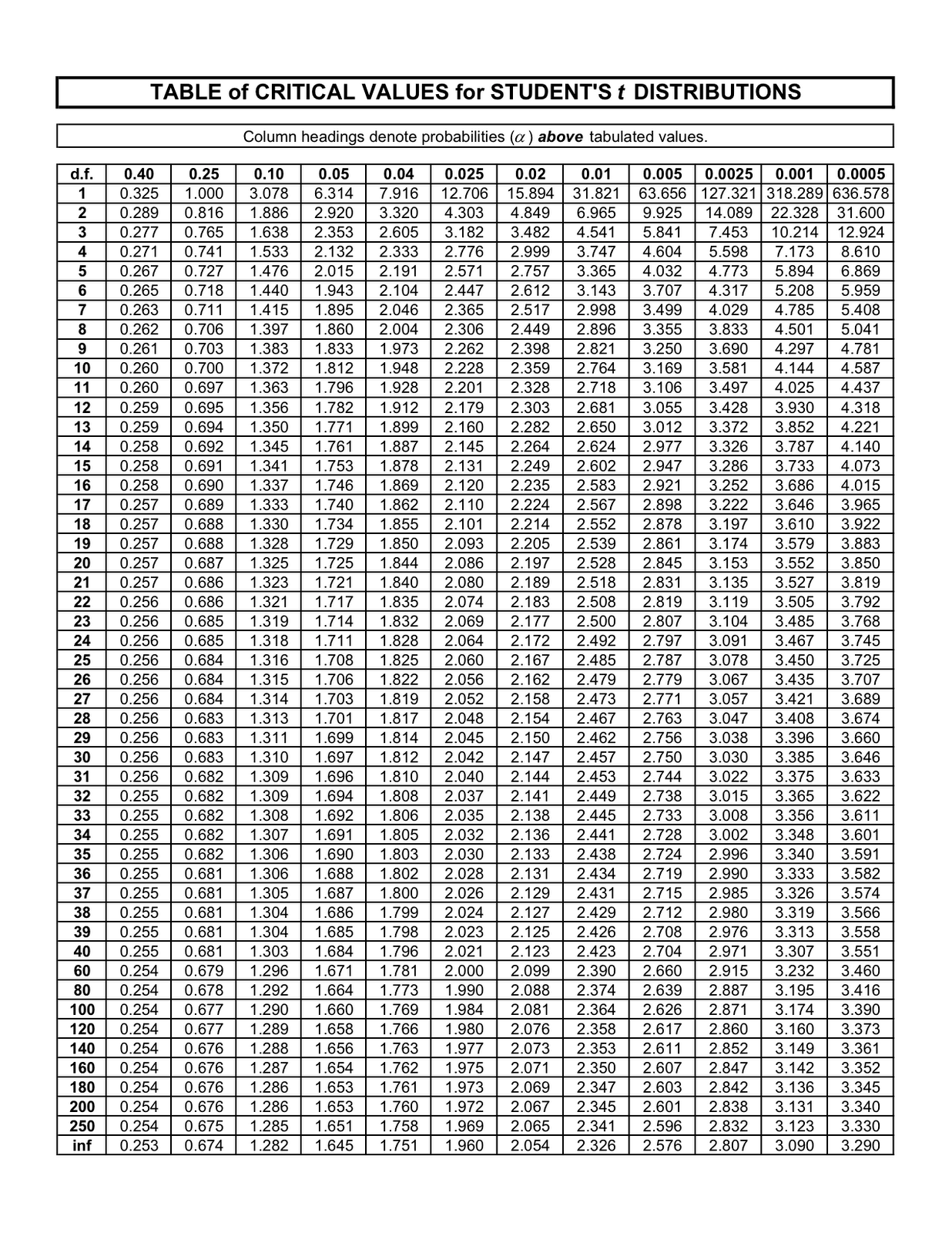
…………Calculating the test statistic from the formula at the NIST webpage is really trivial; the difficulty is in finding proper tables of the T-distribution to interpret the statistic with. The equation for the two-sided test is quite similar to the familiar Z-Score, except that we take the maximum value of the absolute deviation (i.e., the data point minus the mean) before dividing by the standard deviation. The one-sided tests for determining if a minimum or maximum value in a dataset is an outlier are only slightly different; in the former we subtract the minimum value from the mean, while in the latter we subtract the mean from the maximum. Since the code is so easy that even a caveman can do it, I decided not to complicate it by adding logic to let the user select which of the three tests to use; I simply return all three in one row, along with the critical regions for each. The formulas for calculating the critical regions at the NIST’s webpage on Grubbs’ Test are more involved, which requires the use of the function in Figure 3. This in turn calls a rather sloppy but effective function to find the correct critical values for the T-distribution, from the lookup tables defined in Figure 1. I haven’t supplied any code to populate them, but this can be easily rectified by using one of the thousands of lookup tables available on the Internet for that distribution. The tricky part was finding a table that was reasonably complete, since many sources begin skipping over deciles around 40 or 50 degrees of freedom; I populated my own from the best source I could find, the “Tables of Critical values of t for Probabilities” at the StatsToDo website. In fact, you may need to tweak the DDL and retrieval code if you use a different source, since my ranges and stopping point of 200 degrees of freedom are derived from that particular source. According to another lookup table (from a Blogspot post by a writer who I’ve been unable to identify to give proper credit) that I didn’t use because it skips some deciles, the values for 200 and 250 are nearly identical except down to the hundredth of percentage points; the next value listed there is for infinity, which varies only a few hundredths of a percentage point from 250. Unlike researchers working with small samples drawn from an unknown population, SQL Server users can often instantly call up millions of records, so using the smaller values of these lookup tables may be of limited utility for our use cases. I only recently learned how to do hypothesis testing, so my standard advice to check my code before putting it into a production environment definitely holds here. The Grubbs Statistic values match the NIST sample results though and could prove useful, by providing a measurement of “the largest absolute deviation from the sample mean in units of the sample standard deviation.”

Figure 1: DDL for the T-Distribution Lookup Tables
CREATE TABLE [Calculations].[CriticalValueRangeTable](
       [ID] [smallint] IDENTITY(1,1) NOT NULL,
       [OneTail] [decimal](5, 4) NULL,
       [TwoTail] [decimal](5, 4) NULL,
 CONSTRAINT [PK_CriticalValueRangeTable] PRIMARY KEY CLUSTERED (
       [ID] ASC)WITH (PAD_INDEX = OFF, STATISTICS_NORECOMPUTE =
OFF, IGNORE_DUP_KEY = OFF, ALLOW_ROW_LOCKS = ON, ALLOW_PAGE_LOCKS = ON) ON [PRIMARY]) ON [PRIMARY]

CREATE TABLE [Calculations].[TDistributionTable](
[ID] [smallint] IDENTITY(1,1) NOT NULL,
[ProbabilityRange1] [decimal](7, 4) NULL,
[ProbabilityRange2] [decimal](7, 4) NULL,
[ProbabilityRange3] [decimal](7, 4) NULL,
[ProbabilityRange4] [decimal](7, 4) NULL,
[ProbabilityRange5] [decimal](7, 4) NULL,
[ProbabilityRange6] [decimal](7, 4) NULL,
[ProbabilityRange7] [decimal](7, 4) NULL,
CONSTRAINT [PK_TDistributionTable] PRIMARY KEY CLUSTERED ([ID] ASC)WITH (PAD_INDEX = OFF, STATISTICS_NORECOMPUTE = OFF, IGNORE_DUP_KEY = OFF, ALLOW_ROW_LOCKS = ON, ALLOW_PAGE_LOCKS = ON) ON [PRIMARY]) ON [PRIMARY]

Figure 2: Function to Look Up Values in the T-Distribution Tables
CREATE FUNCTION [Calculations].[FindCriticalRegionForTDistributionFunction]
(@DegreesOfFreedom bigint, @SidedTestType bit, @ProbabilityValue decimal(5,4))
RETURNS decimal(7, 4)
AS
BEGIN
DECLARE @CriticalRegion decimal(7, 4)
— this is a little more awkward than I’d like, but hey
      SELECT @CriticalRegion = CASE WHEN ProbabilityRangeColumnID = 1 THEN (SELECT ProbabilityRange1
FROM Calculations.TDistributionTable WHERE ID = (CASE WHEN @DegreesOfFreedom
>= 200 THEN 200 WHEN ID = @DegreesOfFreedom THEN @DegreesOfFreedom ELSE NULL END))
      WHEN ProbabilityRangeColumnID = 2 THEN (SELECT ProbabilityRange2
FROM Calculations.TDistributionTable WHERE ID = (CASE WHEN @DegreesOfFreedom
>= 200 THEN 200 WHEN ID = @DegreesOfFreedom THEN @DegreesOfFreedom
ELSE NULL END))
       WHEN ProbabilityRangeColumnID = 3 THEN (SELECT ProbabilityRange3
FROM Calculations.TDistributionTable WHERE ID = (CASE WHEN @DegreesOfFreedom
>= 200 THEN 200 WHEN ID = @DegreesOfFreedom THEN @DegreesOfFreedom ELSE NULL END))
       WHEN ProbabilityRangeColumnID = 4 THEN (SELECT ProbabilityRange4
FROM Calculations.TDistributionTable WHERE ID = (CASE WHEN @DegreesOfFreedom
>= 200 THEN 200 WHEN ID = @DegreesOfFreedom THEN @DegreesOfFreedom ELSE NULL END))
       WHEN ProbabilityRangeColumnID = 5 THEN (SELECT ProbabilityRange5
FROM Calculations.TDistributionTable WHERE ID = (CASE WHEN @DegreesOfFreedom
>= 200 THEN 200 WHEN ID = @DegreesOfFreedom THEN @DegreesOfFreedom ELSE NULL END))
      WHEN ProbabilityRangeColumnID = 6 THEN (SELECT ProbabilityRange6
FROM Calculations.TDistributionTable WHERE ID = (CASE WHEN @DegreesOfFreedom >= 200 THEN 200 WHEN ID = @DegreesOfFreedom THEN @DegreesOfFreedom ELSE NULL END))
       WHEN ProbabilityRangeColumnID = 7 THEN (SELECT ProbabilityRange7
FROM Calculations.TDistributionTable WHERE ID = (CASE WHEN @DegreesOfFreedom >= 200 THEN
200 WHEN ID = @DegreesOfFreedom THEN @DegreesOfFreedom ELSE NULL END))
       ELSE NULL END
      FROM   (SELECT TOP 1 ID AS ProbabilityRangeColumnID
             FROM  (SELECT ID, ValueRange, ABS(ValueRange – @ProbabilityValue) AS RangeDifference, Lead(ValueRange, 1, 0) OVER (ORDER BY ValueRange) AS Lead
                     FROM (SELECT ID, ‘ValueRange’ = CASE WHEN @SidedTestType = 0 THEN OneTail
                           WHEN @SidedTestType = 1 THEN TwoTail
                           ELSE NULL END
                     FROM [Calculations].[CriticalValueRangeTable] ) AS T1) AS T2
              ORDER BY RangeDifference ASC) AS T3
      RETURN @CriticalRegion
END

Figure 3: Grubbs Hypothesis Testing Function
CREATE FUNCTION [Calculations].[GrubbsHypothesisTestSP](
@DegreesofFreedom bigint, @TestType bit = 0, @SignificanceLevel decimal(38,35))
RETURNS decimal(38,32)
AS
BEGIN
       DECLARE @CriticalValue decimal(38,32), — *** look this up in a table by the SignificanceLevel I’ve already  recalculated according to the formulas, and also the Degrees of Freedom – 2
      @ReturnValue decimal(38,32)
       SELECT @CriticalValue = [Calculations].[FindCriticalRegionForTDistributionFunction] (@DegreesofFreedom, @TestType, @SignificanceLevel)
      SELECT @ReturnValue = Power(Power(@CriticalValue, 2) / (@DegreesOfFreedom – 2
+ Power(@CriticalValue, 2)), 0.5) * ((@DegreesOfFreedom –1) / Power(@DegreesOfFreedom,
0.5))
       RETURN @ReturnValue
END

Figure 4: Code for the the Grubbs Test Procedure
CREATE PROCEDURE [Calculations].[GrubbsTestSP]
@DatabaseName as nvarchar(128) = NULL, @SchemaName as nvarchar(128), @TableName as nvarchar(128),@ColumnName AS nvarchar(128), @DecimalPrecision AS nvarchar(50), @Alpha decimal(38,35) = 0.05
AS

DECLARE @SchemaAndTableName nvarchar(400), @SQLString nvarchar(max)
SET @DatabaseName = @DatabaseName + ‘.’
SET @SchemaAndTableName = ISNull(@DatabaseName, ”) + @SchemaName + ‘.’ + @TableName –I’ll change this value one time, mainly for legibility purposes

SET @SQLString = ‘DECLARE @Mean decimal(‘ + @DecimalPrecision + ‘),
@StDev decimal(‘ + @DecimalPrecision + ‘),
@Min decimal(‘ + @DecimalPrecision + ‘),
@Max decimal(‘ + @DecimalPrecision + ‘),
@GrubbsVersion1 decimal(‘ + @DecimalPrecision + ‘),
@GrubbsVersion2 decimal(‘ + @DecimalPrecision + ‘),
@GrubbsVersion3 decimal(‘ + @DecimalPrecision + ‘),
@DegreesofFreedom bigint,
@SignificanceLevel decimal(‘ + @DecimalPrecision + ‘),
@SignificanceLevelOneSided decimal(‘ + @DecimalPrecision + ‘)

SELECT @DegreesofFreedom=Count(‘ + @ColumnName + ‘), @Mean = Avg(CAST(‘ + @ColumnName + ‘ AS Decimal(‘ + @DecimalPrecision + ‘))), @StDev = StDev(CAST(‘ + @ColumnName + ‘ AS Decimal(‘ + @DecimalPrecision + ‘))), @Min = Min(‘ + @ColumnName + ‘), @Max = Max(‘ + @ColumnName + ‘) FROM ‘ + @SchemaAndTableName + ‘ WHERE ‘ + @ColumnName + ‘ IS NOT NULL

— the sample exercise at the NIST webpage uses a straight value of @SignificanceLevel = @Alpha, rather than the two calculations for two- and one-sided tests that are recommended elsewhere on the directions; hence Ive commented them out for now
–-SET @SignificanceLevel  = ‘ + CAST(@Alpha AS nvarchar(50)) + ‘ / (2 * @DegreesofFreedom)
–SET @SignificanceLevelOneSided = ‘ + CAST(@Alpha AS nvarchar(50)) + ‘ / (@DegreesofFreedom)
SET @SignificanceLevel = ‘ +
CAST(@Alpha AS nvarchar(50)) + ‘
SET @SignificanceLevelOneSided = ‘ + CAST(@Alpha AS nvarchar(50)) + ‘

SELECT @GrubbsVersion1 = Max(‘ + @ColumnName + ‘ – @Mean) / @StDev, @GrubbsVersion2 = ((@Mean – @Min) / @StDev),
@GrubbsVersion3 = ((@Max – @Mean) / @StDev)
FROM ‘ + @SchemaAndTableName +
‘WHERE ‘ + @ColumnName + ‘ IS NOT NULL

SELECT @GrubbsVersion1 AS  GrubbsTwoSided, CAST([Calculations].[GrubbsHypothesisTestSP] (@DegreesOfFreedom, 1, @SignificanceLevel) AS decimal(‘ + @DecimalPrecision + ‘)) AS
CriticalRegionForGrubbsTwoSided,
@GrubbsVersion2 AS  GrubbsLowerOneSided, @GrubbsVersion3 AS  GrubbsUpperOnesided, CAST([Calculations].[GrubbsHypothesisTestSP] (@DegreesOfFreedom, 0, @SignificanceLevelOneSided)  AS decimal(‘ + @DecimalPrecision + ‘)) AS CriticalRegionForGrubbsUpperOneSided‘
–SELECT @SQLString — uncomment this to debug string errors
EXEC (@SQLString)

…………Thankfully, we will be able to reuse the mass of T-SQL in the first three figures in next week’s tutorial, which also requires looking up T-distribution values. The code in Figure 4 will look familiar if you’ve been following this mistutorial series. As always, you’ll have to add the brackets and program in the logic yourself if you allow spaces in your object names; you may also need to add SQL injection and other security code. Also, keep in mind that I’m still using a Calculations schema for these sample routines, so you may need to create one in your database or change the name as needed. The first three parameters allow you to run the procedure against any column in any database for which you have the requisite permissions and access. The @DecimalPrecision also allows you to manually set the precision and scale for the internal calculations of the procedure, in order to avoid arithmetic overflows. There are some slight differences between the parameters of this procedure and those discussed in the last few articles though, such as the fact that the usual @OrderByCode and @PrimaryKeyName are not needed here. The @Alpha parameter allows you to set the significance level of the test to any value you please (including incorrect ones, since I haven’t added any validation code) like the default of 0.05, which corresponds to a 95 percent confidence level. Oddly, Grubbs wrote in the 1969 paper that the confidence levels ought to be at least 99 percent for use with this test, but still used the standard 95 percent in his own example. Similarly, the NIST webpage says to use @Alpha divided by the degrees of freedom for a one-sided test and divided by twice the degrees of freedom for a two-sided test, yet uses a plain significance value of @Alpha = 0.05 in its sample data. Hence the commenting out of the code that would change the @SignificanceLevel to the alternate values. When run against the sample exercise on the NIST page, my code is accurate within about a hundredth of a percentage point, as long as this adjustment is made.

Figure 5: Results for the Grubbs Test Procedure
EXEC   Calculations.GrubbsTestSP
            @DatabaseName =N’DataMiningProjects’,
             @SchemaName= N’Health’,
             @TableName = N’DuchennesTable’,
             @ColumnName= N’PyruvateKinase’,
             @DecimalPrecision= N’12,7′,
             @Alpha = 0.05

 

 

…………Executing a query like the one above against the Duchennes dataset we’ll be working with in this tutorial series produced the five columns above. The first, third and fourth columns represent the Grubbs Statistics for the two-sided, minimum and maximum tests respectively, while the Critical Regions are derived from the aforementioned code in Figures 1 through 3. The Grubbs Statistics are far beyond the critical regions, so yes, the maximum values in the dataset are beyond the thresholds and thus can be defined as “outliers.” Keep in mind that after testing the procedure against several different columns in different datasets, I’ve only seen slight differences between the two-sided result and the upper one-sided; due to lack of appropriate samples to work through, I cannot say whether or not that can be expected or is an error on my part. The PyruvateKinase column refers to an enzyme that is apparently involved in the devastating Duchennes form of muscular dystrophy, which is the subject of a tiny nine-kilobyte sample dataset made publicly available by Vanderbilt University’s Department of Biostatistics. In the last couple of blog posts I used the first float column of the Higgs Boson Dataset that the University of California at Irvine’s Machine Learning Repository has made available online, which occupies nearly 6 gigabytes of space in the DataMiningProjects database I’ve created to encompass all of the practice datasets I’ll be using in tutorial series to come. Traversing that much space in index scans and seeks turned out to be somewhat costly for the two versions of Z-Scores that I coded in the last two posts, but I haven’t bothered to post Client Statistics from SQL Server Management Studio (SSMS) because the Grubbs’ Test procedure takes only a matter of seconds, even for the massive float columns of the Physics.HiggsBosonTable.
…………The procedure may perform well compared to other outlier detection methods, but its usefulness is limited. I have yet to test it against a table that didn’t turn out to have outliers – which is likely to be the case for most of the large tables that DBAs might run the procedure on. Grubbs’ Test is more useful for the kind of small tables used in hypothesis testing, rather than exploratory data mining and data quality analyses, which are far more common uses cases in the SQL Server user community. Statistical testing of this kind is also prone to several real dangers I’ve touched on in the last few articles and others that I have yet to address. The confidence levels commonly associated with them are pretty much drawn out of thin air; you’ll see 95 percent used most of the time, but only because it was an arbitrary de facto standard long before the UNIVAC. There really isn’t a good justification for it, except for the fact that it has been used for so long. Secondly, probabilities are not guarantees; there is a finite chance that random fluctuations alone could produce a dataset that consisted of nothing but outliers, using any definition and detection method. Worst of all, Grubbs’ Test requires a Gaussian (i.e.”normal”) distribution, i.e. the bell curve. Without goodness-of-fit tests that clearly demonstrate that the data ought to fit the normal distribution, such tests are useless – or worse, deceptive. As Grubbs himself puts it mildly, “Until such time as criteria not sensitive to the normality assumption are developed, the experimenter is cautioned against interpreting the probabilities too literally when normality of the data is not assured.” I don’t yet know how to apply some of the best goodness-of-fit tests (mainly because I’m still having trouble wrapping my head around some of the intricacies of cumulative distribution functions) but that won’t stop me from harping on this point repeatedly: the extent to which statistics are bandied about in many academic disciplines without proper testing today is simply alarming. The one place we can least afford to see them is in medical research, where they become a matter of life and death, but at least half of all studies published today contain at least one statistical error. The most common error appears to be the lack of goodness-of-fit testing; researchers in many fields seem to be in the habit of routinely applying tests that depend on a Gaussian distribution with reckless disregard for their validity. It’s not surprising that this occurs, given that there are so few statistical tests that can be used with the scores of other distributions that data might follow. If researchers everywhere were held to a proper standard of evidence, they might not be able to back up claims for a favorite project or experimental medicine with any statistics at all.
…………This leads straight back to the logical and moral issues that I’ve tried to reiterate throughout this series: there are an awful lot of shenanigans that go on with “lies, damned lies and statistics,” as the old saying goes. Grubbs’ Test is no more vulnerable to misuse than any other measure based on the normal distribution, all of which can be invalid, misleading or worse when the data is not naturally Gaussian. It is sometimes, however, applied recursively by simply deleting outliers until some stopping criteria is reached, which raises the grim possibility of improper handling of unfavorable data points. In some situations, an iterative Grubbs Test is vulnerable to false negatives, in which actual outliers are not detected, or false positives, in which haphazard definitions of stopping criteria lead to the deletion of good data. That brings us back full circle to the confluence of subjective definitions, “moving the goalposts” and inadequate analysis of the causes of aberrance which I discussed at length in the last article. Thankfully, the Generalized Extreme Studentized Deviate Test (GESD) ameliorates some of the standard problems associated with the sequential application of Grubbs’ Test by making a few adjustments; the NIST recommends that either the GESD or the Tietjen-Moore test be applied when looking for more than one outlier, which is almost always going to be the case in a SQL Server database. The math and code for both are also relatively simple. Unfortunately, they are both dependent on a Gaussian distribution, which means they also require goodness-of-fit tests that are often dispensed with in an irresponsible manner. The same limitation applies to Dixon’s Q-Test, which is simple to code, as well as to Chauvenet’s Criterion, which is not. It may also be true of Peirce’s Criterion, which will also be featured later in this series. Interquartile Range is a much more easily coded method of outlier detection which also may be less dependent on the normal distribution. Later in the series, I’ll give a quick recap of the Clustering algorithm in SQL Server Data Mining (SSDM) and supply some eye candy that is much easier on the brain than these fancy equations in Visual Outlier Detection with SQL Server Reporting Services. Towards the end I’ll delve into more difficult methods like Cook’s Distance and the Modified Thompson Tau Test, then Mahalanobis Distance. Many of these more sophisticated methods are of course more difficult to code than GESD, Tietjen-Moore and Dixon’s Q-Test, but they may also be more applicable to distributions besides the bell curve.

Outlier Detection with SQL Server, part 2.2: Modified Z-Scores

By Steve Bolton

…………There are apparently many subtle variations on Z-Scores, a ubiquitous measure that is practically a cornerstone in the foundation of statistics. The popularity and ease of implementation of Z-Scores are what made me decide to tackle them early on in this series of amateur self-tutorials, on using various components of SQL Server to detect those aberrant data points we call “outliers.” As discussed in the last two posts, there are many different means of identifying outliers, which may be understood best by categorizing them by their use cases; the right choice of detection tools is essentially a function of the questions one wants to ask of the data, the number and types of inputs, the desired mathematical properties of the outputs and in between, the performance and other requirements used in transforming the inputs into outputs. From my scant understanding of what little literature I’ve read on the topic, statisticians and other researchers commonly encounter use cases where the sensitivity of ordinary measurements to outliers has to be toned down, often in response to fat-tailed (i.e. highly skewed) distributions. The Modified Z-Scores developed by Temple University Prof. Boris Iglewicz and University of Massachusetts Prof. David C. Hoaglin are one means of adjusting Z-Scores for such cases, but hardly the only one. I’m highlighting it merely because I was introduced to it early on, while trying to learn the subject of stats from the National Institute for Standards and Technology’s Engineering Statistics Handbook, one of the best online resources for anyone trying to wade through this notoriously dry subject.[I]
                Iglewicz and Hoaglin suggest specific cut-off criteria for their measure, that can of course be adjusted as needed by users – which raises the whole question of researchers “moving the goalposts” or setting them haphazardly when using any means of outlier detection. Correct classification is a thorny issue with every method we’ll discuss in this series; I’m merely using the hard boundary associated with Modified Z-Scores as an introduction to the all-important topic of subjectivity in category definitions. As an amateur, I can’t give any guidance on whether or not to use a specific cut-off point for classifying outliers, although it would seem to be common sense that more detailed rough and fuzzy sets ought to be more commonly used in place of hard limits than they are. It is worth reiterating that outliers also vary significantly in their causes and the responses made to them, not just the means of differentiation. The frequent mismatches between the causes and responses and the lack of attention paid to discerning them both leave the door wide open to innumerable fallacies and sometimes outright fraud, which as I discussed earlier in this series, is frighteningly common in certain fields. The definition of an outlier is subjective, depending on the kind of investigation a researcher chooses to perform, but whether or not a particular data point meets the chosen criteria is wholly objective. Fallacies and fraud arise when the distinction in the right uses and proper places of subjectivity and objectivity are blurred; the whole history of human philosophy demonstrates that when the former is loosed from such bonds, the result is always maniacal madness. For example, a person can choose to affix the name “pepperoni pizza” to anything they want; but once they’ve set tomato sauce, bread, cheese and the like as part of the criteria, then they can’t pretend that a pencil sharpener or a Planck length fits the definition, because whether or not they consist of the same ingredients set forth in the criteria is an objective matter. That’s plain common sense, which suddenly becomes uncommon when the labeler has an incentive to fudge their definitions, or worse yet, a pedantic justification for it, like solipsism (i.e., one of the major symptoms of schizophrenia). Outlier detection presents a serious temptation to simply ignore the distinctions between causes and put no effort to differentiating the correct response to others, so that data miners and others who use these tools frequently just delete records that don’t fit their models and theories, or adjust their definitions of the term to achieve the same purpose. I’ll delve into outlier deletion in more depth a few posts from now, but the issue of subjective limits can serve as a transition into my usual dire disclaimer that math formulas, including those underpinning data mining algorithms and outlier detection, resides in a Pandora’s Box. The Modified Z-Scores under discussion today do not open the box any wider than any other formula; this is merely the context in which all statistical measures naturally reside, in which the slightest logical deviation in their use may lead to erroneous, misleading or even fraudulent conclusions. Data mining tools can be used quite easily by amateurs like myself for exploratory data analysis, but need to be handled like scalpels when attempting to prove a specific point. Nevertheless, they’re often employed carelessly like sledge hammers by professionals in many different fields, particularly health care. The specter of fallacious reasoning hems us in all sides, and wielding these tools properly for this purpose requires more skill than the old board game of Operation. The difference with math and logic is that there is no buzzer to warn us when we’ve used them wrong; there may be terrible consequences down the line in the form of falling bridges and adverse medical reactions, but the intelligentsia also has the intellectual power to explain those away using the same poor reasoning. What is called for here is not intelligence, but wisdom; without it, outlier detection methods merely prove the old adage, “There are three kinds of lies: lies, damned lies and statistics.”[ii] No data mining tool or math formula is going to going to provide a quick fix for this overarching problem, which hangs like a Sword of Damocles over everything that researchers, scientists, mathematicians and data miners do; the only fix is to apply the use of reason rigorously, which requires a deep understanding of logical fallacies and in turn, painful self-examination. Neither I nor most of the DBAs who read this probably have that kind of training, so our use cases ought to be limited to exploratory analysis – which can be a highly productive exercise, even for the unqualified – rather than hypothesis testing and the like.
…………The point of using Modified Z-Scores is to address situations where it is desirable to reduce the sensitivity to outliers, so that there are for all intents and purposes fewer false positives when classifying them. Whether or not such reduced sensitivity is a wise choice to fit the problem at hand is one question; whether or not Modified Z-Scores succeed in doing so seems to be an open and shut case. In this series I’m trying to grasp the mechanisms that make these algorithms and formulas work as they do, which is something I didn’t delve into adequately in my series on SQL Server Data Mining (SSDM). The reason why Iglewicz and Hoaglin’s Z-Scores are less sensitive to outliers without being completely blind to them is that they use medians rather than means, which are an alternate measure of central tendency that is known for being less affected by unusual values. Both medians and means are basically primordial forms of clustering that identify a specific location near the center of a dataset, but the former is less affected by the most distant points. The formula given at the NIST website is not all that difficult to decipher or code in T-SQL; I was unable to get ahold of a copy of their original paper to see what the reasoning was behind the constant that appears in it, but it is child’s play to simply include it in the code and be done with it.[iii]  This was my first introduction to median absolute deviation (MAD), which is a variation of the average absolute deviation that is even less affected by extremes in the tail because the data in the tails have less influence on the calculation of the median than they do on the mean.”[iv] I initially confused it with a more common calculation, mean absolute deviation because of the similar names. The idea is basically the same though: instead of taking a mean of a mean, we compare each data point to the median of the whole dataset, then calculate a new median for the absolute value of those distances. Then we take subtract the median from each data point again and multiply that result by a constant, 0.6745, the divide the result by the MAD. The equations are actually quite easy to read; most of the T-SQL involved in implementing them is dedicated to calculating the two medians, using some subqueries and windowing functions. I’ve precalculated both in Common Table Expressions (CTEs) at the beginning of this week’s T-SQL stored procedure, because this reduces them to one-time operations (I think the technical term might an “Θ(n) operation”) and makes the complicated dynamic SQL a little more legible. The T-SQL in Figure 1 could be streamlined further to suit your needs by removing the DENSE_RANK calculation, the OutlierCandidate column and the @OrderByCode logic, which are dispensable elements I’ve added as conveniences.

Figure 1: Code for the Modified Z-Score Stored Procedure[v]
CREATE PROCEDURE [Calculations].[ModifiedZScoreSP]
@DatabaseName as nvarchar(128) = NULL, @SchemaName as nvarchar(128), @TableName as nvarchar(128),@ColumnName AS nvarchar(128), @PrimaryKeyName as nvarchar(400), @OrderByCode as tinyint = 1, @DecimalPrecision AS nvarchar(50)–1 is by PK ASC, 2 is by
PK Desc, 3  is by ColumnName ASC, 4 is by ColumnName DESC, 5  is by ZScore ASC, 6 is by ZScore DESC
AS

SET @DatabaseName = @DatabaseName + ‘.’
DECLARE @SchemaAndTableName nvarchar(400), @SQLString nvarchar(max)
SET @SchemaAndTableName = ISNull(@DatabaseName, ”) + @SchemaName + ‘.’ + @TableName –I’ll change
this value one time, mainly for legibility purposes

SET @SQLString =
‘DECLARE @OrderByCode as tinyint ,– pass the outer value like a parameter of sorts
@Median AS decimal(‘ + @DecimalPrecision + ‘),
@MedianAbsoluteDeviation AS decimal(‘ + @DecimalPrecision + ‘)

— PRECALCULATED STATS
————————–
— precalculating these 3 stats not only makes the code more legible, but is more efficient because it is a one-time operation
– first get the median

WITH MedianCTE
(‘ + @ColumnName + ‘, RN, DenseRank)
AS
(
SELECT ‘ + @ColumnName + ‘, RN, DENSE_RANK() OVER (PARTITION BY 1 ORDER BY RN DESC) AS DenseRank
FROM (SELECT ‘ + @ColumnName + ‘, ROW_NUMBER() OVER (ORDER BY ‘ + @ColumnName + ‘) AS RN
     FROM ‘ + @SchemaAndTableName + ‘
WHERE ‘ + @ColumnName + ‘ IS NOT NULL) AS T1
)

SELECT @Median = Avg(‘ + @ColumnName + ‘) FROM MedianCTE WHERE RN BETWEEN DenseRank – 1 AND DenseRank +1;

— get the MedianAbsoluteDeviation
WITH MedianAbsoluteDeviationCTE
(‘ + @ColumnName + ‘, RN, DenseRank)
AS
(
SELECT NewMedian, RN, DENSE_RANK() OVER
(PARTITION BY 1 ORDER BY RN DESC) AS DenseRank
FROM        (SELECT NewMedian, ROW_NUMBER() OVER (ORDER BY NewMedian) AS RN
       FROM             (SELECT ABS(‘ + @ColumnName + ‘ – @Median) AS NewMedian
              FROM ‘ + @SchemaAndTableName + ‘
              WHERE ‘ + @ColumnName + ‘ IS NOT NULL) AS T1) AS T2)

SELECT @MedianAbsoluteDeviation = Avg(‘ + @ColumnName + ‘)
FROM MedianAbsoluteDeviationCTE
WHERE RN BETWEEN DenseRank – 1 AND DenseRank +1;

–SELECT @Median
–SELECT @MedianAbsoluteDeviation
SET @OrderByCode = ‘ + CAST(@OrderByCode  AS nvarchar(50) ) + ‘

— OUTLIER COMPARISON OPERATIONS
— now check each data point
SELECT ‘ + @PrimaryKeyName + ‘, ‘ + @ColumnName + ‘, ModifiedZScore, DENSE_RANK () OVER (ORDER BY ModifiedZScore) AS GroupRank,
”OutlierCandidate” = CASE WHEN Abs(ModifiedZScore) > 3.5 THEN 1
       ELSE 0
       END
FROM (SELECT ‘ + @PrimaryKeyName + ‘, ‘ + @ColumnName + ‘, ((0.6745 * (‘ + @ColumnName + ‘ – @Median)) / @MedianAbsoluteDeviation) AS ModifiedZScore
FROM ‘ + @SchemaAndTableName + ‘) AS T1
       ORDER BY
CASE WHEN @OrderByCode = 1 THEN ‘ + @PrimaryKeyName + ‘ END ASC,
CASE WHEN @OrderByCode = 2 THEN ‘ + @PrimaryKeyName + ‘ END DESC,
CASE WHEN @OrderByCode = 3 THEN ‘ + @ColumnName + ‘ END ASC,
CASE WHEN @OrderByCode = 4 THEN ‘ + @ColumnName + ‘ END DESC,
CASE WHEN @OrderByCode = 5 THEN ModifiedZScore
END ASC,
CASE WHEN @OrderByCode = 6 THEN ModifiedZScore END DESC’
–SELECT @SQLString — uncomment this to debug string errors
EXEC (@SQLString)

…………Note that I’m using almost all of the same parameters and dynamic SQL format as in the article on regular Z-Scores. The combination of the first three parameters allows you to execute the procedure against any table in any database, assuming you have the requisite permissions. Just like in the last tutorial, the @OrderByCode parameter allows you to sort the results by 1) the primary key values, ascending; 2) the primary key value descending; 3) the column values ascending; 4) the column values descending; 5) the Modified Z-Score ascending and 6) the Modified Z-Score descending. You’ll have to supply your own @DecimalPrecision values and tweak them to avoid arithmetic overflows, which are tricky to handle when multiple calculations can change the number of decimal places repeatedly. I usually try setting these values to the original precision and scale of decimal and numeric columns if they’re high enough, but when working with integers you’ll have to decide how many decimal places are appropriate for your output.  You can debug the dynamic SQL by uncommenting the next-to-last line and two others beginning with comment marks and SELECTS. I’ve also used DENSE_RANK windowing function again to assign identical results to specific groups by their Modified Z-Score values, which comes in handy with columns that have few distinct values that are repeated many times. The OutlierCandidate is merely a bit column that reveals whether or not the ModifiedZScore falls outside the ±3.5 threshold set by Iglewicz and Hoaglin. Your requirements may be different, so feel free to change the threshold or eliminate it altogether; it wouldn’t be all that difficult either to replace hard thresholds like this with more flexible fuzzy set criteria with graded memberships. If you use @OrderByCode 5 or 6, values where OutlierCandidate = 1 will be sorted to the top and bottom of the results. As usual, you’ll have to add your own brackets and logic to handle spaces if you allow them in your object names (I have a ruthless ban on them in my own code, for legibility purposes) and program in your own security to handle risks like SQL injection.

Figure 2: Results for Column1 of the HiggsBosonTable
EXEC [Calculations].[ModifiedZScoreSP]
              @DatabaseName = N’DataMiningProjects’,
             @SchemaName = N’Physics’,
              @TableName = N’HiggsBosonTable’,
              @ColumnName = N’Column1′,
              @PrimaryKeyName = N’ID’,
             @OrderByCode = 6,
              @DecimalPrecision = N’33,29′

 

Figure 3: Client Statistics for the Modified Z-Scores Procedure

…………In last week’s tutorial, I tested my Z-Score stored procedure on the first float column of a nearly 6-gigabyte table from the Higgs Boson Dataset, which is made publicly available by the University of California at Irvine’s Machine Learning Repository. In future mistutorials I will use a dataset on the Duchennes form of muscular dystrophy provided by Vanderbilt University’s Department of Biostatistics, as well as transcriptions of the Voynich Manuscript, a creepy tome whose medieval author encrypted it so well that no one has been able to crack it since, including the National Security Agency (NSA). For the sake of consistency, I tested my Modified Z-Scores procedure against the same Higgs Boson column. Using the query at the top of Figure 2 returned the corresponding results, plus about 11 million more rows that I somehow couldn’t cram into the article. There were some records at the very bottom with Modified Z-Scores near -1, but none that qualified for Iglewicz and Hoaglin’s cut-off point for outliers.
…………I didn’t bother to post screenshots of the execution plans because they weren’t pretty, nor would they fit on an NFL scoreboard. The novel approach I took of comparing the middle point of two windowing functions moving in opposite directions added a lot of expensive sorts, which even the addition of a non-clustered index couldn’t fix. As depicted in Figure 3, the index improved the Client Processing Time and Total Execution Time significantly, but the procedure still consumed far too much memory on my poor beat-up development machine and took too long for my tastes. It will do just fine on columns in small tables, but expect it to take a while if you’re executing it on 11 million rows of a 6-gig database using an outdated workstation in place of a real server.
…………That drawback ought to refocus attention on one of the caveats I want to stress in this series: I’m posting these articles because I don’t know what I’m doing and want to learn, not because I have any real expertise. As with my series A Rickety Stairway to SQL Server Data Mining, I’m passing on my misadventures so that others don’t repeat them. Another error I rectified along the way was accidentally substituting a mode for the median while wool-gathering; that procedure might actually be useful in catching certain outliers and I will post it if anyone thinks they can benefit, but the bottom line is that I almost posted an article based on the wrong formula. Just keep in mind that my code samples in this series will always need further testing before going into a production environment. Consider these posts an introduction to the topic, not the last word. If all goes according to plan, I’ll be introducing both myself and my readers to Chauvenet’s Criterion, which is a means of outlier detection that is intrinsically dependent on a Gaussian distribution. I may follow these up by going on a tangent with some fairly easy means of outlier detection, like Grubbs’ Test and the Tietjen-Moore Test, the Generalized Extreme Studentized Deviate (ESD) Test, Interquartile Range and Dixon’s Q-Test. At some point I’ll also get into a discussion of Visual Outlier Detection with Reporting Services (featuring a lot of eye candy) and do a quick recap of Clustering with SSDM. Towards the end of the series I’ll tackle Cook’s Distance the Modified Thompson Tau Test, then end with the daunting task of coding Mahalanobis Distance. I hope to use that last post as a springboard towards a much longer and more difficult series months down the line, Information Measurement with SQL Server.

[i] That’s more “dry humor,” but not as bad as the hydrology joke in the last column.

[ii] Although frequently attributed to Mark Twain and Benjamin Disraeli, the quip apparently originated with British politician Leonard H. Courtney in 1895. See the TwainQuotes webpage “Statistics” at http://www.twainquotes.com/Statistics.html.

[iii] See “Detection of Outliers,” an undated article published at the National Institute for Standards and Technology’s Engineering Statistics Handbook website. Available online at http://www.itl.nist.gov/div898/handbook/eda/section3/eda35h.htm. The page in turn cites Iglewicz, Boris and Hoaglin, David, 1993, “Volume 16: How to Detect and Handle Outliers,” The ASQC Basic References in Quality Control: Statistical Techniques, Edward F. Mykytka, Ph.D., Editor.

[iv] See “Measures of Scale,” an undated article published at the National Institute for Standards and Technology’s Engineering Statistics Handbook website. Available online at http://www.itl.nist.gov/div898/handbook/eda/section3/eda356.htm#MAD

[v]  While coding this, I forgot how to use modulo properly and made use of See Byers, Mark, 2009, response to the thread “How Can I Determine is Digit Even Number?” published Nov. 26, 2009 at StackOverflow.com. Available online at http://stackoverflow.com/questions/1805420/how-can-i-determine-is-digit-even-number.  I also double-checked my median calculations against the MathIsFun webpage “How to Find the Median Value” at http://www.mathsisfun.com/median.html.